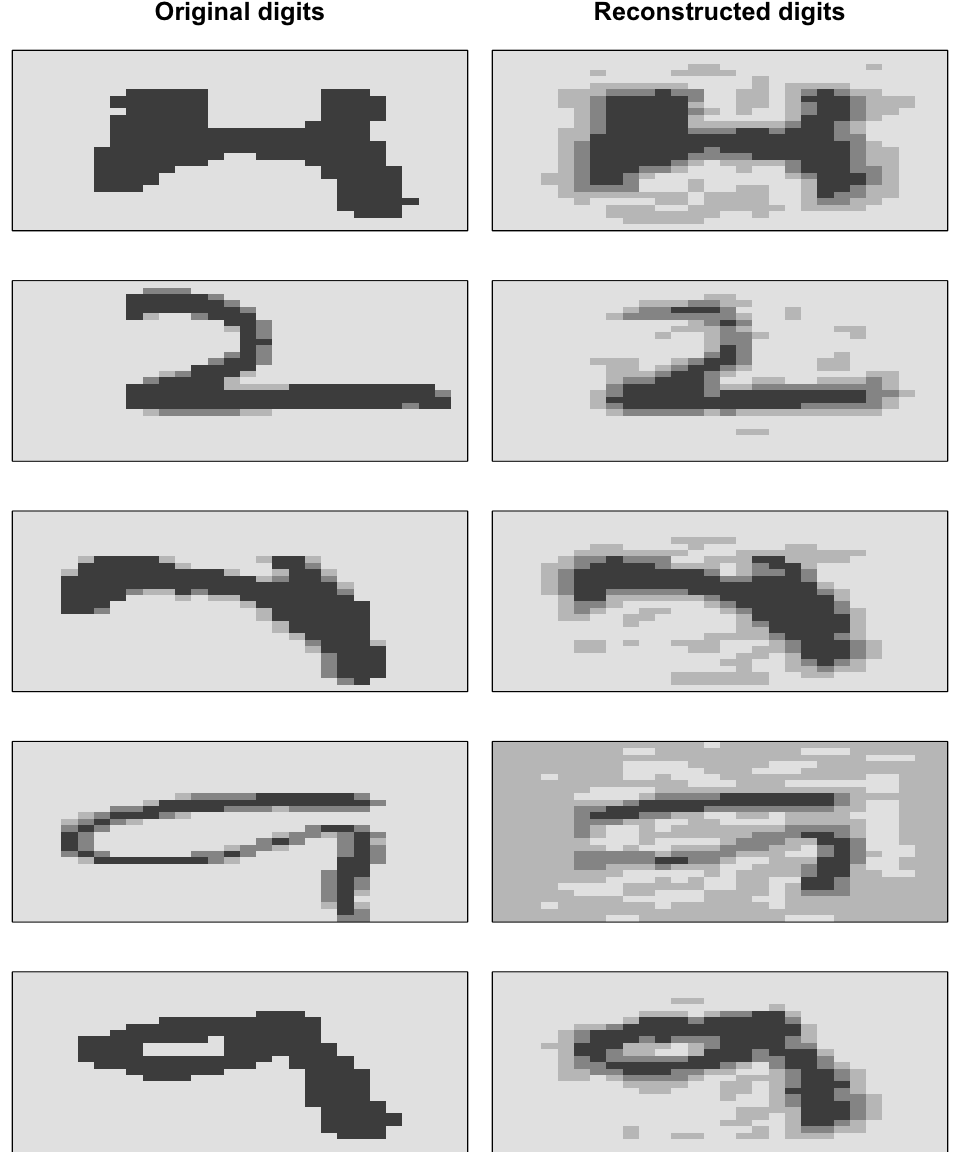
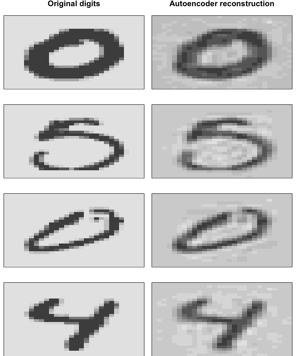
19.4 Undercomplete autoencoders

As the goal is to create a reduced set of codings that adequately represents \(X\) the number of neurons is less than the number of inputs which helps to capture the most dominant features and signals in the data.

19.4.1 Comparing PCA to an autoencoder

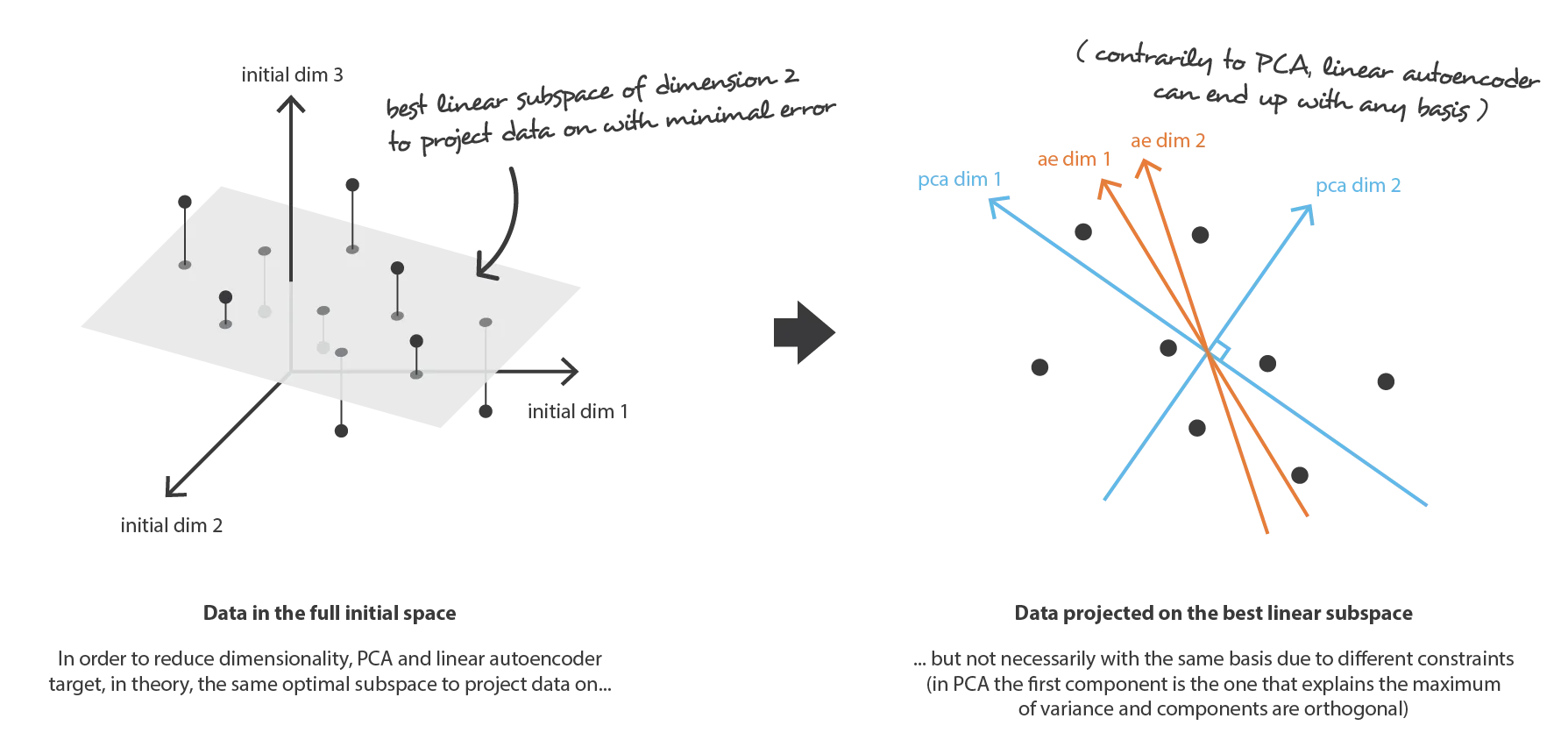
When an autoencoder uses only linear activation functions and MSE as loss function, then it can be shown that the autoencoder reduces to PCA.

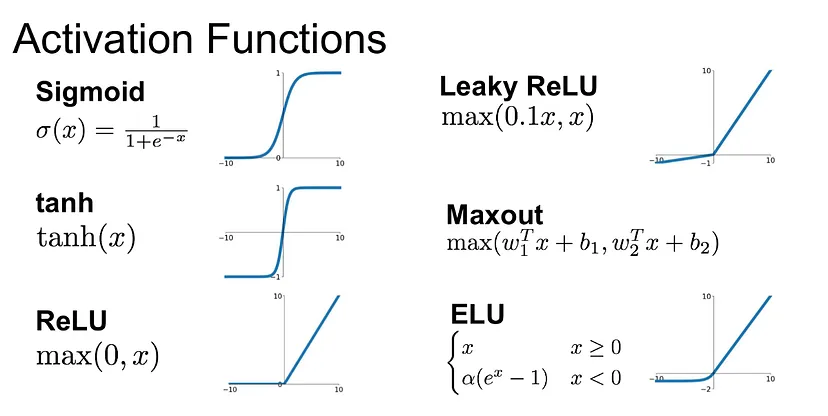
But when nonlinear activation functions are used, autoencoders provide nonlinear generalizations of PCA. Here you can see some activation functions:

As we can see bellow, now it is easier to see the difference between groups.

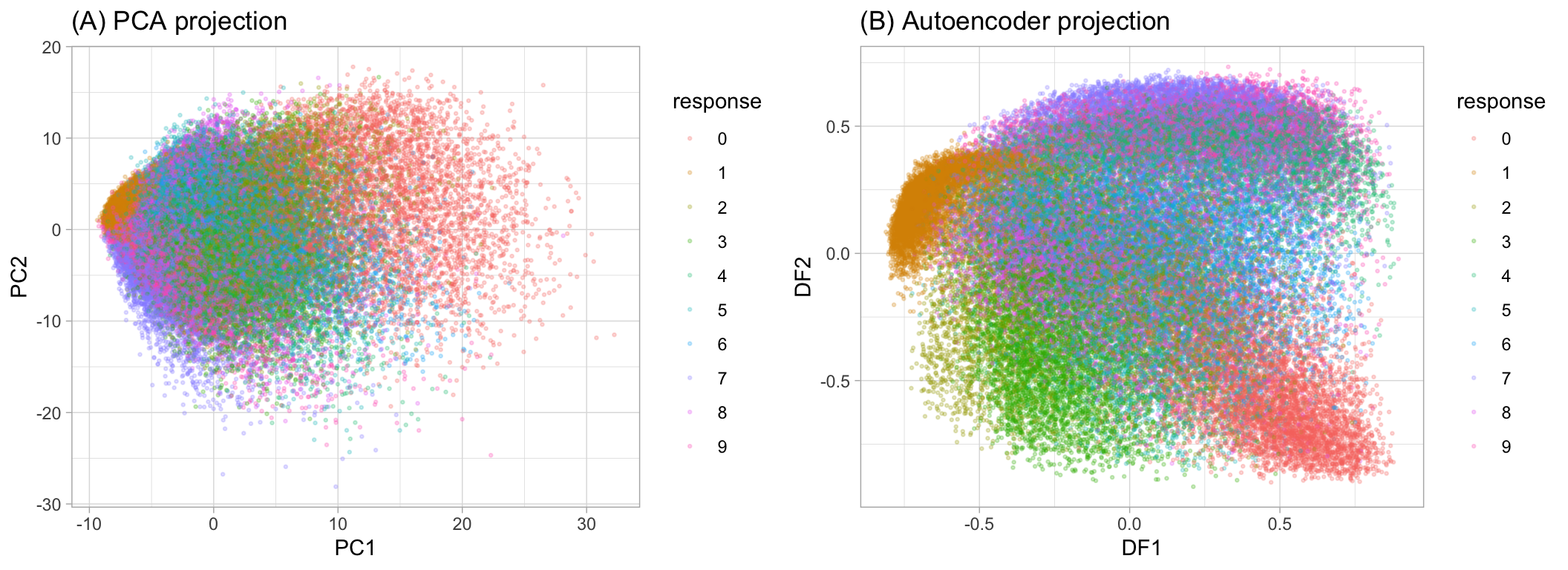
MNIST response variable projected onto a reduced feature space

But we need to be aware that some of the new components can be correlated.

19.4.2 Coding example

Let’s train an autoencoder with h2o.

features <- as.h2o(mnist$train$images)

ae1 <- h2o.deeplearning(

  # Names or indices of the predictor variables 
  x = seq_along(features),
  
  # Training data
  training_frame = features,
  
  # Sets the network as a autoencoder
  autoencoder = TRUE,
  
  # A single hidden layer with only two codings
  hidden = 2,
  
  # Defining activation function
  activation = 'Tanh',
  
  # As 80% of the elements in the MNIST data set are zeros
  # we can speed up computations by defining this option
  sparse = TRUE
  
)

Now we can extract the deep features from the trained autoencoder.

ae1_codings <- h2o.deepfeatures(ae1, features, layer = 1)
ae1_codings
##     DF.L1.C1    DF.L1.C2
## 1 -0.1558956 -0.06456967
## 2  0.3778544 -0.61518649
## 3  0.2002303  0.31214266
## 4 -0.6955515  0.13225607
## 5  0.1912538  0.59865392
## 6  0.2310982  0.20322605
## 
## [60000 rows x 2 columns]

19.4.3 Stacked autoencoders

They have multiple hidden layers to represent more complex, nonlinear relationships at a reduced computational cost and often yield better data compression.

As you can see bellow, they typically follow a symmetrical pattern.

19.4.4 Tuning hidden layers configuration

1. Creating a grid with different configurations for the hidden layers.

hyper_grid <- list(hidden = list(
  c(50),
  c(100), 
  c(300, 100, 300),
  c(100, 50, 100),
  c(250, 100, 50, 100, 250)
))

2. Training a model for each option

ae_grid <- h2o.grid(
  algorithm = 'deeplearning',
  x = seq_along(features),
  training_frame = features,
  grid_id = 'autoencoder_grid',
  autoencoder = TRUE,
  activation = 'Tanh',
  hyper_params = hyper_grid,
  sparse = TRUE,
  ignore_const_cols = FALSE,
  seed = 123
)

3. Identifying the best option.

h2o.getGrid('autoencoder_grid', sort_by = 'mse', decreasing = FALSE)
## H2O Grid Details
## ================
## 
## Grid ID: autoencoder_grid 
## Used hyper parameters: 
##   -  hidden 
## Number of models: 5 
## Number of failed models: 0 
## 
## Hyper-Parameter Search Summary: ordered by increasing mse
##                     hidden                 model_ids                  mse
## 1                    [100] autoencoder_grid3_model_2  0.00674637890553651
## 2          [300, 100, 300] autoencoder_grid3_model_3  0.00830502966843272
## 3           [100, 50, 100] autoencoder_grid3_model_4 0.011215307972822733
## 4                     [50] autoencoder_grid3_model_1 0.012450109189122541
## 5 [250, 100, 50, 100, 250] autoencoder_grid3_model_5 0.014410280145600972

4. Selecting the best model

best_model_id <- ae_grid@model_ids[[1]]
best_model <- h2o.getModel(best_model_id)

5. Validating output layers results visually

# Get sampled test images
index <- sample(1:nrow(mnist$test$images), 4)
sampled_digits <- mnist$test$images[index, ]
colnames(sampled_digits) <- paste0("V", seq_len(ncol(sampled_digits)))

# Predict reconstructed pixel values
reconstructed_digits <- predict(best_model, as.h2o(sampled_digits))
names(reconstructed_digits) <- paste0("V", seq_len(ncol(reconstructed_digits)))

# Combining results
combine <- rbind(
  sampled_digits, 
  as.matrix(reconstructed_digits)
)

# Plot original versus reconstructed
par(mfrow = c(1, 3), mar=c(1, 1, 1, 1))
layout(matrix(seq_len(nrow(combine)), 4, 2, byrow = FALSE))
for(i in seq_len(nrow(combine))) {
  image(matrix(combine[i, ], 28, 28)[, 28:1], xaxt="n", yaxt="n")
}

19.4.5 Anomaly detection

Based on reconstruction error, we can find observations have feature attributes that differ significantly from the other features and can be considered as unusual or outliers.

1. Get the reconstruction error.

(reconstruction_errors <- h2o.anomaly(best_model, features))
##   Reconstruction.MSE
## 1        0.009879666
## 2        0.006485201
## 3        0.017470110
## 4        0.002339352
## 5        0.006077669
## 6        0.007171287
## 
## [60000 rows x 1 column]

2. Plotting the distribution with a histogram or boxplot.

reconstruction_errors <- as.data.frame(reconstruction_errors)
ggplot(reconstruction_errors, aes(Reconstruction.MSE)) +
  geom_histogram()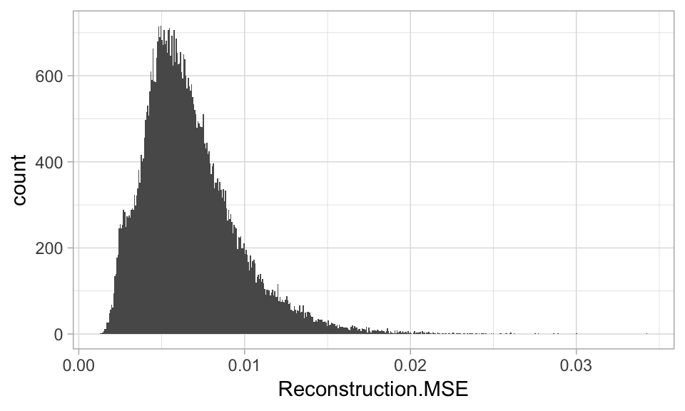

3. Retrain the autoencoder on a subset of the inputs that represent high quality inputs like the observations under the 75-th percentile of reconstruction error.

4. Select the observations with the highest reconstruction error.