3.2 Target engineering

Transforming the response (target) variable can lead to predictive improvement, especially with parametric models (i.e., models with certain assumptions about the underlying distribution of response and predictor variables). Let’s use the AMES housing dataset to illustrate this concept.

First look at train dataset.

ames_train %>% 
     select(1:10) %>% 
     glimpse()

## Rows: 2,049
## Columns: 10
## $ Sale_Price   <int> 105500, 88000, 120000, 125000, 67500, 112000, 122000, 127…
## $ MS_SubClass  <fct> Two_Story_PUD_1946_and_Newer, Two_Story_PUD_1946_and_Newe…
## $ MS_Zoning    <fct> Residential_Medium_Density, Residential_Medium_Density, R…
## $ Lot_Frontage <dbl> 21, 21, 24, 50, 70, 68, 0, 0, 98, 80, 87, 60, 70, 68, 60,…
## $ Lot_Area     <int> 1680, 1680, 2280, 7175, 9800, 8930, 9819, 6897, 13260, 99…
## $ Street       <fct> Pave, Pave, Pave, Pave, Pave, Pave, Pave, Pave, Pave, Pav…
## $ Alley        <fct> No_Alley_Access, No_Alley_Access, No_Alley_Access, No_All…
## $ Lot_Shape    <fct> Regular, Regular, Regular, Regular, Regular, Regular, Sli…
## $ Land_Contour <fct> Lvl, Lvl, Lvl, Lvl, Lvl, Lvl, Lvl, Lvl, Lvl, Lvl, Lvl, Lv…
## $ Utilities    <fct> AllPub, AllPub, AllPub, AllPub, AllPub, AllPub, AllPub, A…

Plot the histogram response variable (Sales_Price)

ames_train %>% 
     ggplot(aes(Sale_Price)) + 
     geom_histogram(fill = 'steelblue')

## `stat_bin()` using `bins = 30`. Pick better value with `binwidth`.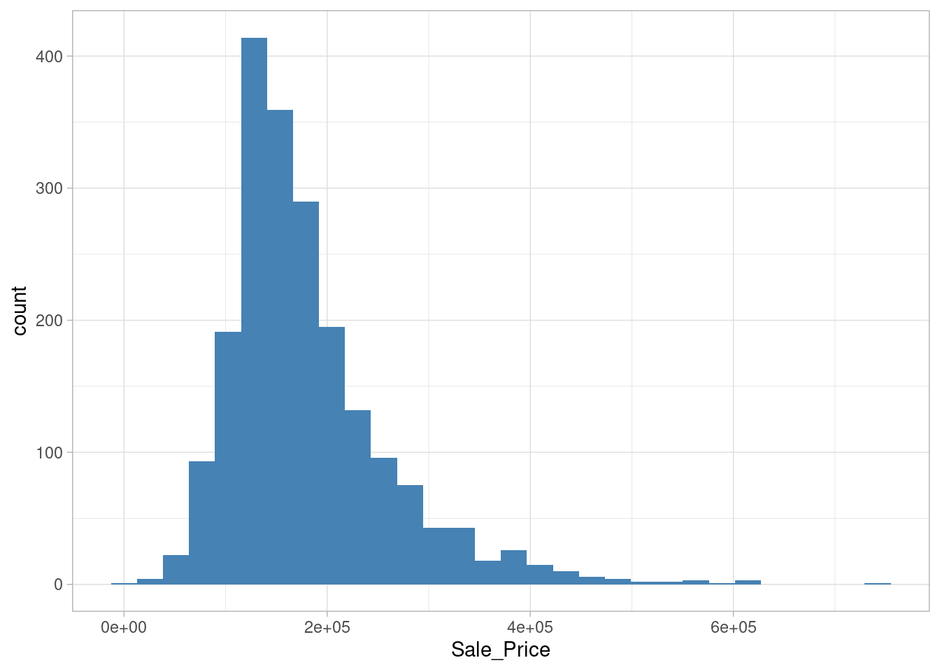

library(moments)

skewness(ames_train$Sale_Price)

## [1] 1.672107

Sale_Price has a right skeweness. This means that the majority of the distribution values are left of the distribution mean.

Solution #1 - Normalize with a log transformation

ames_train %>% 
     mutate(log_Sale_Price = log(Sale_Price)) %>% 
     ggplot(aes(log_Sale_Price)) + 
     geom_histogram(fill = 'steelblue')

## `stat_bin()` using `bins = 30`. Pick better value with `binwidth`.

skewness(log(ames_train$Sale_Price))

## [1] -0.09635868

Solution #2 - Apply Box-Cox transformation

lambda  <- forecast::BoxCox.lambda(ames_train$Sale_Price)

## Registered S3 method overwritten by 'quantmod':
##   method            from
##   as.zoo.data.frame zoo

ames_train %>% 
     mutate(bc_Sale_Price = forecast::BoxCox(ames_train$Sale_Price, lambda)) %>% 
     ggplot(aes(bc_Sale_Price)) + 
     geom_histogram(fill = 'steelblue')

## `stat_bin()` using `bins = 30`. Pick better value with `binwidth`.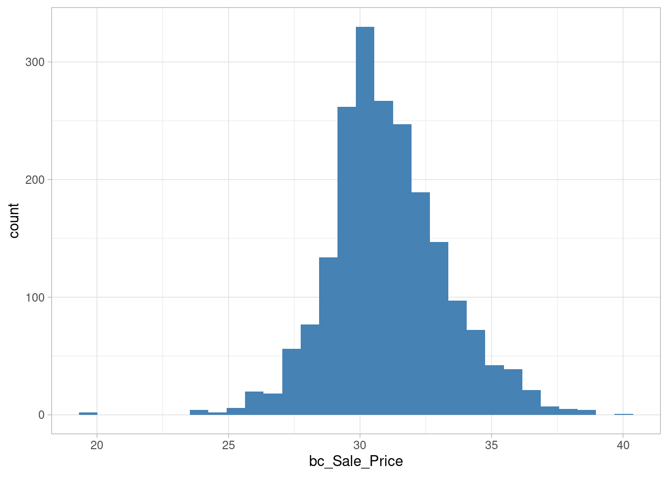

skewness(forecast::BoxCox(ames_train$Sale_Price, lambda))

## [1] 0.2001352

Comments from the textbook:

• Be sure to compute the lambda on the training set and apply that same lambda to both the training and test set to minimize data leakage. The recipes package automates this process for you.

• If your response has negative values, the Yeo-Johnson transformation is very similar to the Box-Cox but does not require the input variables to be strictly positive. To apply, use step_YeoJohnson().