16.8 Feature interactions
Most of the relationships between features and some response variable are complex and include interactions, but identifying and understanding the nature of these interactions can be a challenge, but a number of recent empirical studies have shown that interactions can be uncovered by flexible models.
Two or more predictors are said to interact if their combined effect is different (less or greater) than what we would expect if we were to add the impact of each of their effects when considered alone.
by Max Kuhn and Kjell Johnson
The interaction strength (\(H\)-statistic or \(\rho\)) is to measure how much of the *variation of the predicted outcome depends on the interaction of the features using the partial dependence values for the features of interest.
- \(\rho = 0\): When there is no interaction at all.
- \(\rho = 1\): If all of variation depends on a given interaction.
We can explore the interaction between:
- A feature and all other features
1. For variable i in {1,...,p} do
     | f(x) = estimate predicted values with original model
     | pd(x) = partial dependence of variable i
     | pd(!x) = partial dependence of all features excluding i (computationally expensive)
     | upper = sum(f(x) - pd(x) - pd(!x))
     | lower = variance(f(x))
     | rho = upper / lower
   End
2. Sort variables by descending rho (interaction strength) - 2 features
1. i = a selected variable of interest
2. For remaining variables j in {1,...,p} do
     | pd(ij) = interaction partial dependence of variables i and j
     | pd(i) = partial dependence of variable i
     | pd(j) = partial dependence of variable j
     | upper = sum(pd(ij) - pd(i) - pd(j))
     | lower = variance(pd(ij))
     | rho = upper / lower
   End
3. Sort interaction relationship by descending rho (interaction strength)
16.8.1 Implementation
A feature and all other features
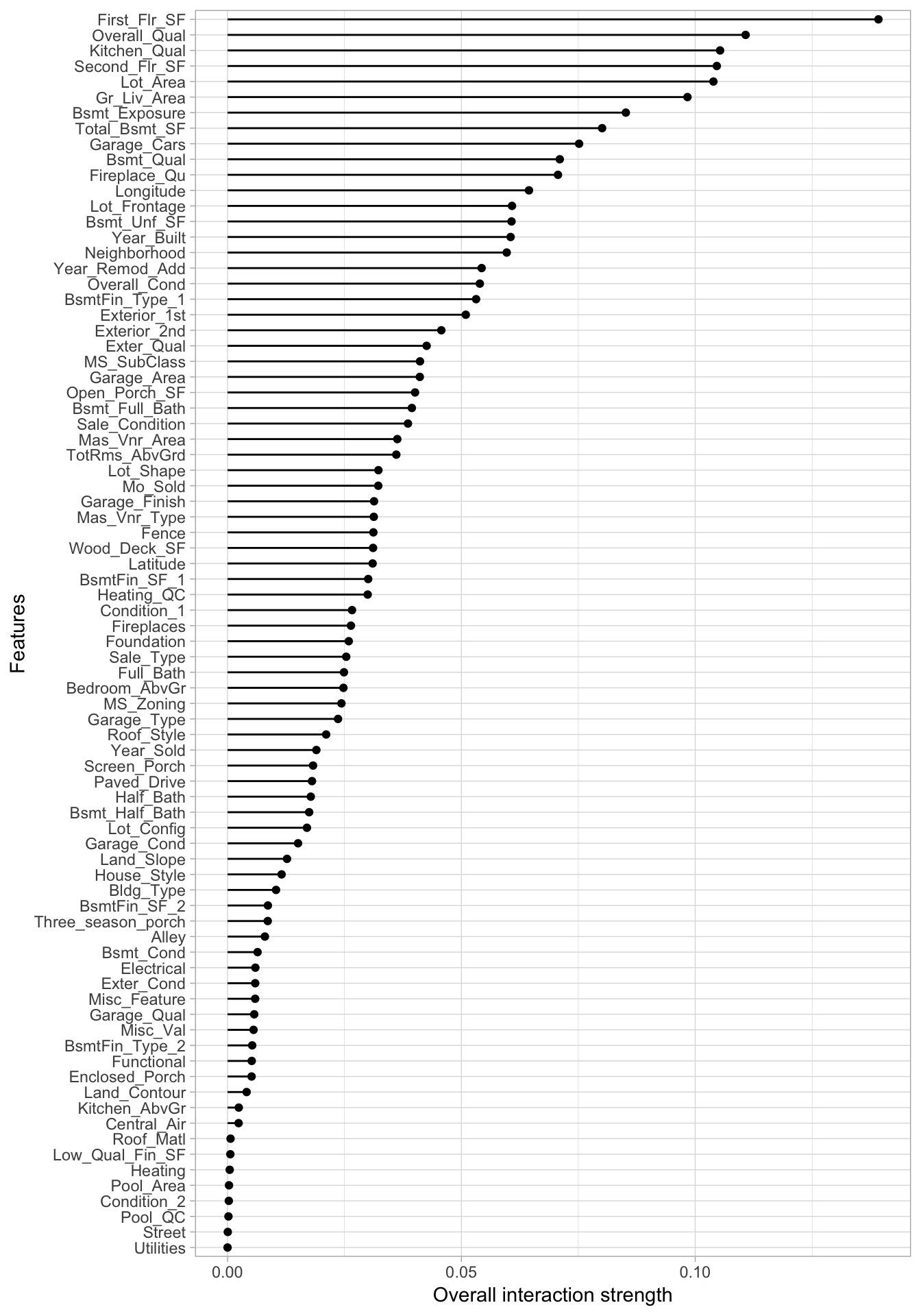
Computing the one-way interaction \(H\)-statistic took two hours to complete
interact <- Interaction$new(components_iml)

interact$results %>%
  arrange(desc(.interaction)) %>%
  head()
##        .feature .interaction
## 1  First_Flr_SF   0.13917718
## 2  Overall_Qual   0.11077722
## 3  Kitchen_Qual   0.10531653
## 4 Second_Flr_SF   0.10461824
## 5      Lot_Area   0.10389242
## 6   Gr_Liv_Area   0.09833997

plot(interact)
2 features
interact_2way <- Interaction$new(components_iml, feature = "First_Flr_SF")

interact_2way$results %>%
  arrange(desc(.interaction)) %>%
  top_n(10)
##                      .feature .interaction
## 1   Overall_Qual:First_Flr_SF   0.14385963
## 2     Year_Built:First_Flr_SF   0.09314573
## 3   Kitchen_Qual:First_Flr_SF   0.06567883
## 4      Bsmt_Qual:First_Flr_SF   0.06228321
## 5  Bsmt_Exposure:First_Flr_SF   0.05900530
## 6  Second_Flr_SF:First_Flr_SF   0.05747438
## 7  Kitchen_AbvGr:First_Flr_SF   0.05675684
## 8    Bsmt_Unf_SF:First_Flr_SF   0.05476509
## 9     Fireplaces:First_Flr_SF   0.05470992
## 10  Mas_Vnr_Area:First_Flr_SF   0.05439255
Interactions and response variable relation
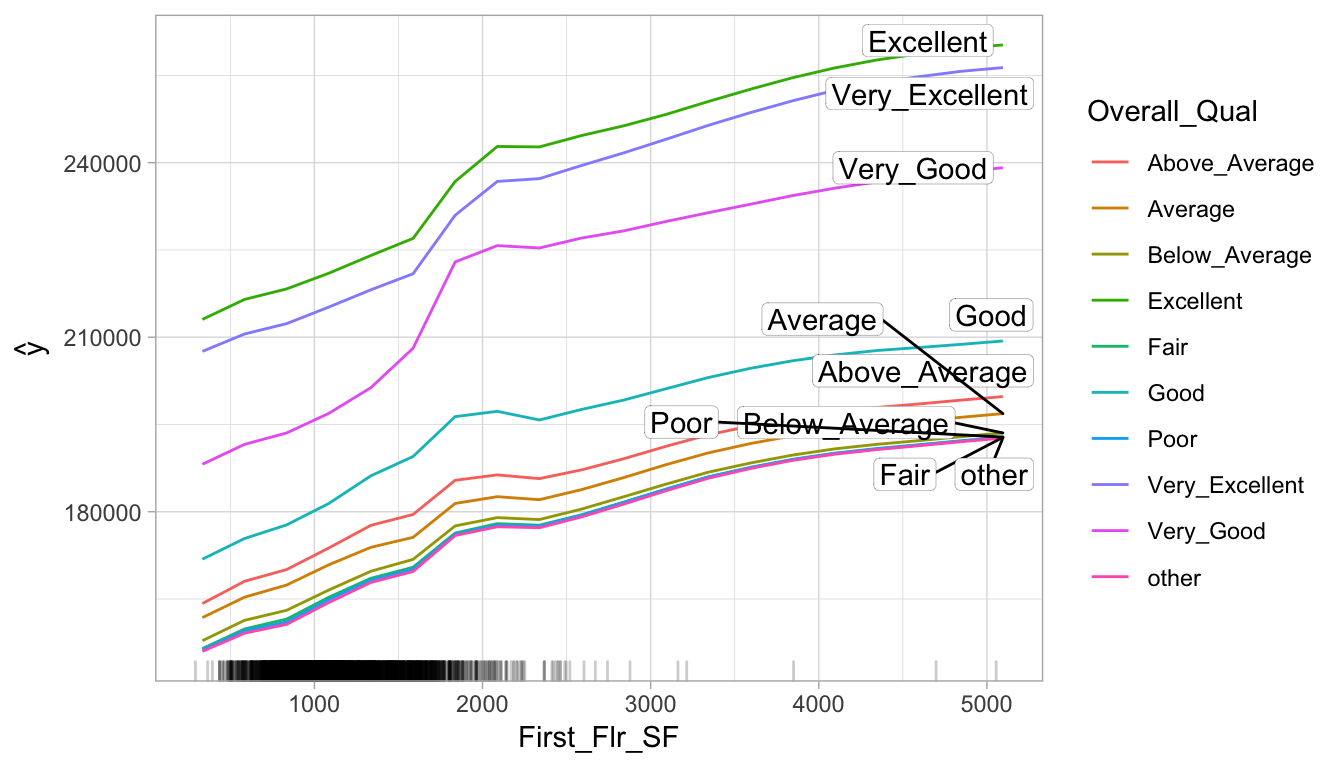
By playing attention to the slope differences we can see that:
Properties with “good” or lower
Overall_Qualvalues tend to level off theirSale_PricesasFirst_Flr_SFincreases, more so than properties with really strongOverall_Qual values.Properties with “very good”
Overall_Qualtend to experience a much larger increase in Sale_Price as First_Flr_SF increases from 1500–2000, compared to most other properties.
interaction_pdp <- Partial$new(
  components_iml,
  c("First_Flr_SF", "Overall_Qual"),
  ice = FALSE,
  grid.size = 20
)
plot(interaction_pdp)
16.8.2 Alternatives
PDP-based variable importance measure implemented in the
vip::vint()function.Max Kuhn and Kjell Johnson give some strategys to find interactions:
Expert-selected interactions should be the first to be explored as they might find complex higher-order interactions.
Brute-Force Approach for data sets that have a small to moderate number of predictors.
- Simple Screening of nested statistical models.
- Penalized Regression
Two-stage Modeling and Guiding Principles
- Start training a model that does not account for interaction effects.
- Based on the results follow on the next strategies to explain the renamining variation using 2-way interactions as three-way and beyond are almost impossible to interpret, rarely capture a significant amount of response variation and we only need a fraction of the possible effects to explain a significant amount of response variation.
- Strong heredity requires that for an interaction to be considered in a model, all lower-level preceding terms must explain a significant amount of response variation.
- Weak heredity relaxes this requirement and would consider any possible interaction with the significant factor.

- Tree-based Methods as each subsequent node can be thought of as representation of a localized interaction between the previous node and the current node.
- Starting training a tree-based model.
- Estimating the predictors’ importance.
- Using must important predictors to validate 2-way interactions using partial depend plots or a simpler model like lineal regression, as tree-based methods will use predictors involved important interactions multiple times throughout multiple trees to uncover the relationship with the response.
node_4 <- I(x1 < 0.655) * I(x2 < 0.5) * I(x2 < 0.316) * 0.939