16.10 Shapley values

This method observes how the prediction changes for each possible subset of features and then combine these changes to form a unique contribution for each feature value.

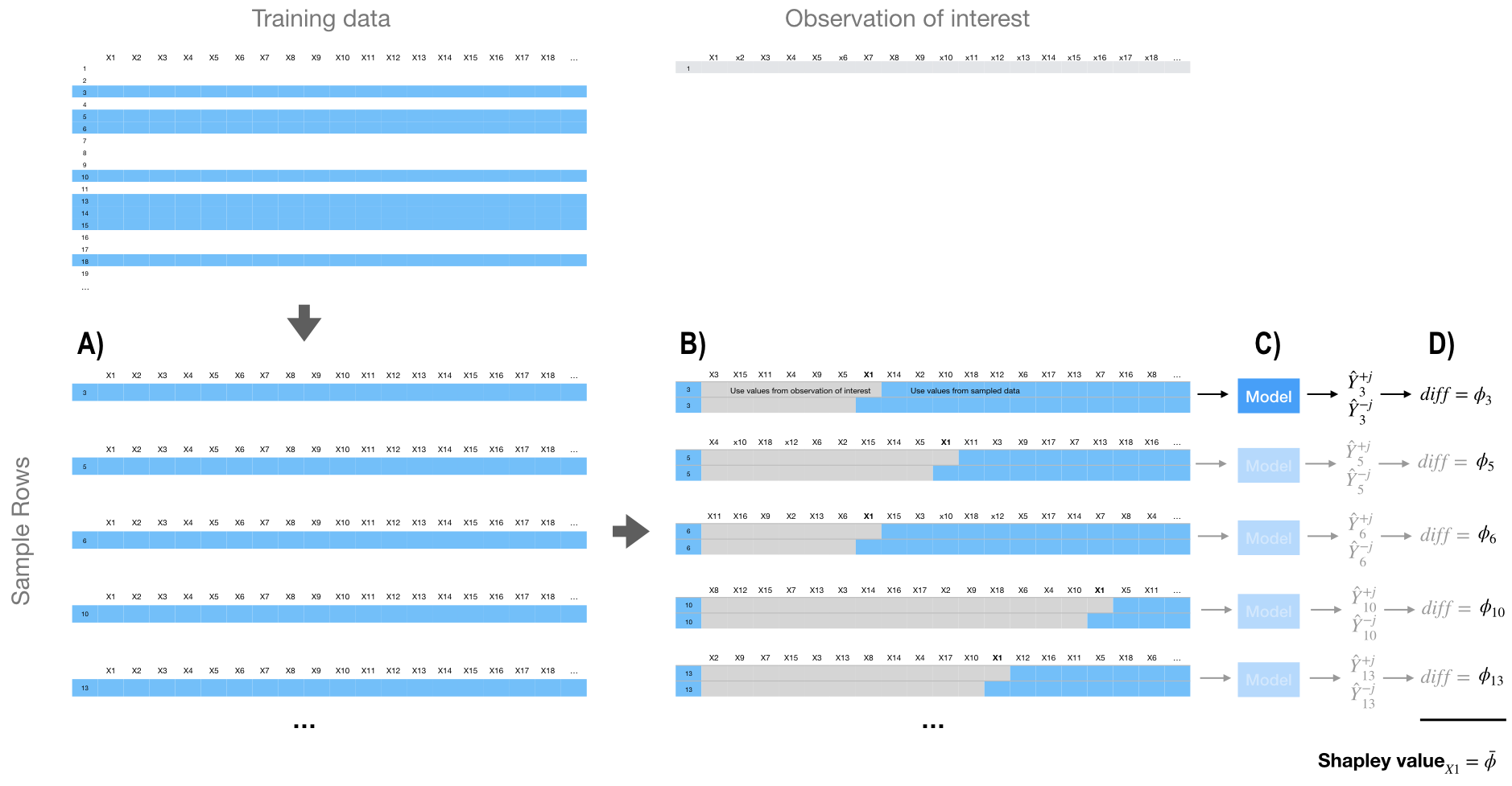
To compute the approximate Shapley contribution of feature \(x_j\) to \(x\) we need to repeat the next process several times (e.g., 10–100) for each feature/observation combination and the results are averaged together.

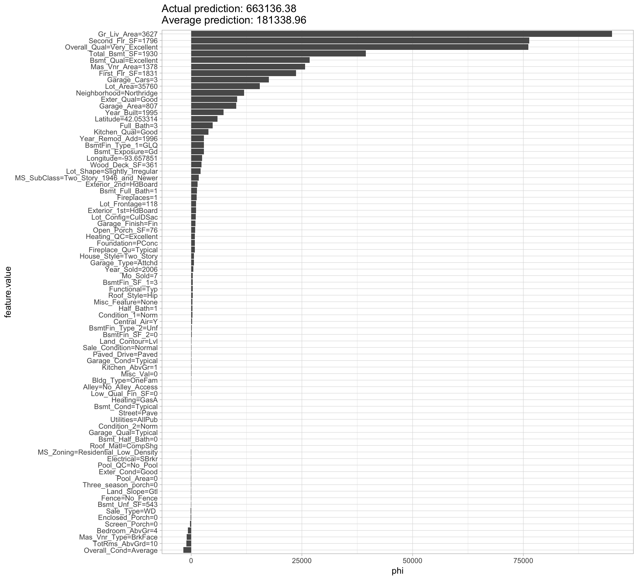
The aggregated Shapley values (\(\phi\) = phi) represent the contribution of each feature towards a predicted value compared to the average prediction for the data set.

A. We sample the training data.

B. We create two copies of an individually sampled row and randomize the order of the features.

Then in one copy we include all values from the observation of interest for the values from the first column feature up to and including \(X_1\). We then include the values from the sampled row for all the other features.
In the second copy, we include all values from the observation of interest for the values from the first column feature up to but not including \(X_1\). We use values from the sample row for \(X_1\) and all the other features.

C. We apply our model to both copies of this row and in step.

D. We compute the difference between the predicted outputs and calculate the mean of random samples.

16.10.1 Implementation

In R the algorithm has been written in iml and fastshap. Let’s use the iml one:

# Compute (approximate) Shapley values
(
  shapley <- Shapley$new(
    components_iml,
    x.interest = high_ob,
    sample.size = 1000
  )
)
## Interpretation method:  Shapley 
## Predicted value: 663136.380000, Average prediction: 181338.963590 (diff = 481797.416410)
## 
## Analysed predictor: 
## Prediction task: unknown 
## 
## 
## Analysed data:
## Sampling from data.frame with 2199 rows and 80 columns.
## 
## Head of results:
##        feature         phi      phi.var
## 1  MS_SubClass  1746.38653 4.269700e+07
## 2    MS_Zoning   -24.01968 3.640500e+06
## 3 Lot_Frontage  1104.17628 7.420201e+07
## 4     Lot_Area 15471.49017 3.994880e+08
## 5       Street     1.03684 6.198064e+03
## 6        Alley    41.81164 5.831185e+05
##                          feature.value
## 1 MS_SubClass=Two_Story_1946_and_Newer
## 2    MS_Zoning=Residential_Low_Density
## 3                     Lot_Frontage=118
## 4                       Lot_Area=35760
## 5                          Street=Pave
## 6                Alley=No_Alley_Access

# Plot results
plot(shapley)

# Reuse existing object
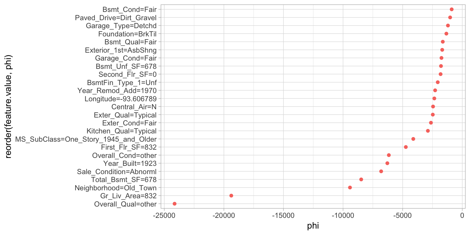
shapley$explain(x.interest = low_ob)

# Plot results
shapley$results %>%
  top_n(25, wt = abs(phi)) %>%
  ggplot(aes(phi, reorder(feature.value, phi), color = phi > 0)) +
  geom_point(show.legend = FALSE)