9.6 - Feature Interpretation
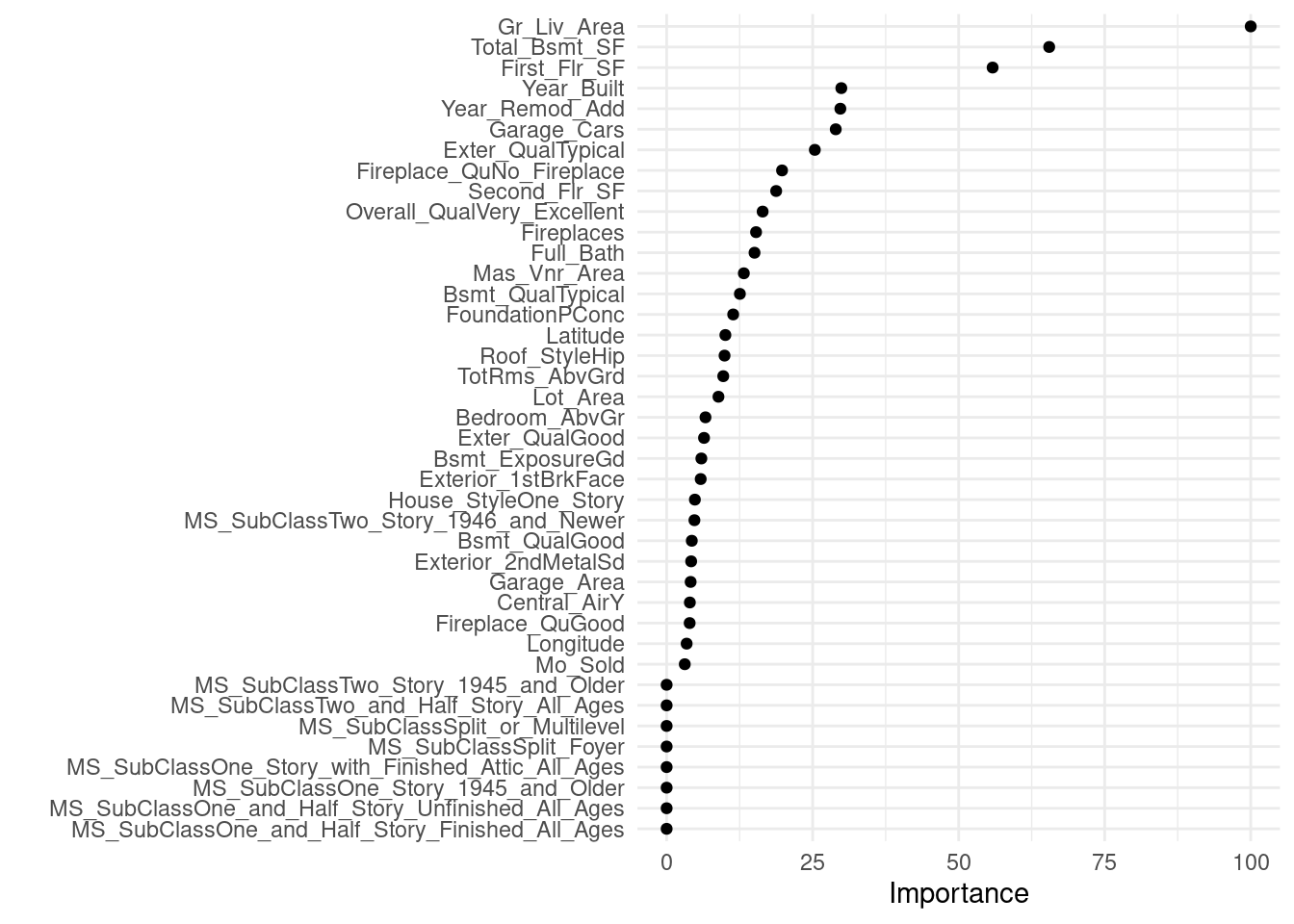
The figure below illustrates the top 40 features in the Ames housing decision tree.
vip(ames_dt3, num_features = 40, geom = 'point')
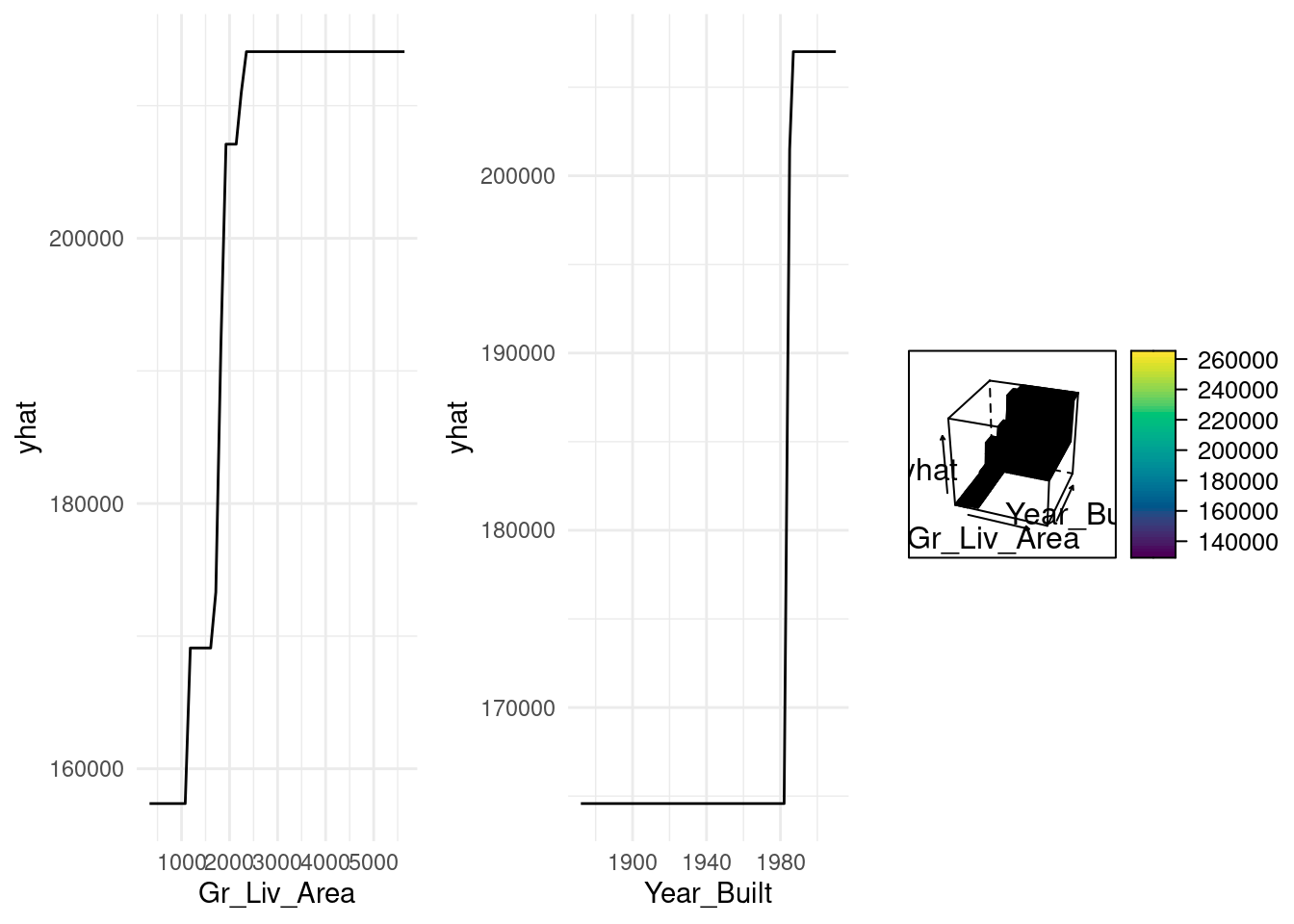
Partial dependency plots
# Construct partial dependence plots
p1 <- partial(ames_dt3, pred.var = "Gr_Liv_Area") %>% autoplot()
p2 <- partial(ames_dt3, pred.var = "Year_Built") %>% autoplot()
p3 <- partial(ames_dt3, pred.var = c("Gr_Liv_Area", "Year_Built")) %>%
  plotPartial(levelplot = FALSE, zlab = "yhat", drape = TRUE,
              colorkey = TRUE, screen = list(z = -20, x = -60))

# Display plots side by side
gridExtra::grid.arrange(p1, p2, p3, ncol = 3)