16.6 Partial dependence
16.6.1 Concept
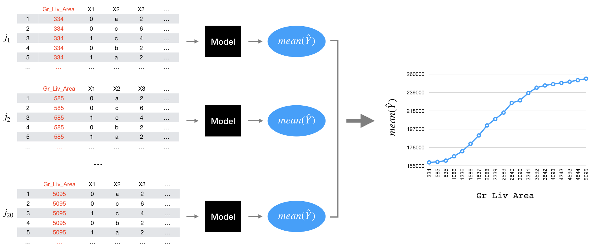
It allows us to understand how the response variable changes as we change the value of a feature while taking into account the average effect of all the other features in the model, when the model has weak interactions between features.
- Splitting the feature of interest into \(j\) equally spaced values. For example, if \(j = 20\) for the
Gr_Liv_Areawe could write the next code.
j_values <-
  seq(from = 334,
      to = 5095,
      length.out = 20L) |>
  round(digits = 2)

matrix(j_values, nrow = 5, byrow = TRUE)
## [,1] [,2] [,3] [,4]
## [1,] 334.00 584.58 835.16 1085.74
## [2,] 1336.32 1586.89 1837.47 2088.05
## [3,] 2338.63 2589.21 2839.79 3090.37
## [4,] 3340.95 3591.53 3842.11 4092.68
## [5,] 4343.26 4593.84 4844.42 5095.00Making \(j\) copies of the original training data.
For each copy setting the
Gr_Liv_Areawith the corresponding value. For example, the value for first copy will be 334 and the second 584.58 until changing the last copy 5095.Predicting the outcome for each observation in each of the \(j\) copies.
Averaging the predicted values for each set.
Plotting the average of each \(j\) value.

16.6.2 Implementation
DALEX
dalex_pdp <- model_profile(explainer = components_dalex,
                           variables = "Gr_Liv_Area",
                           N = 20L)

dalex_pdp

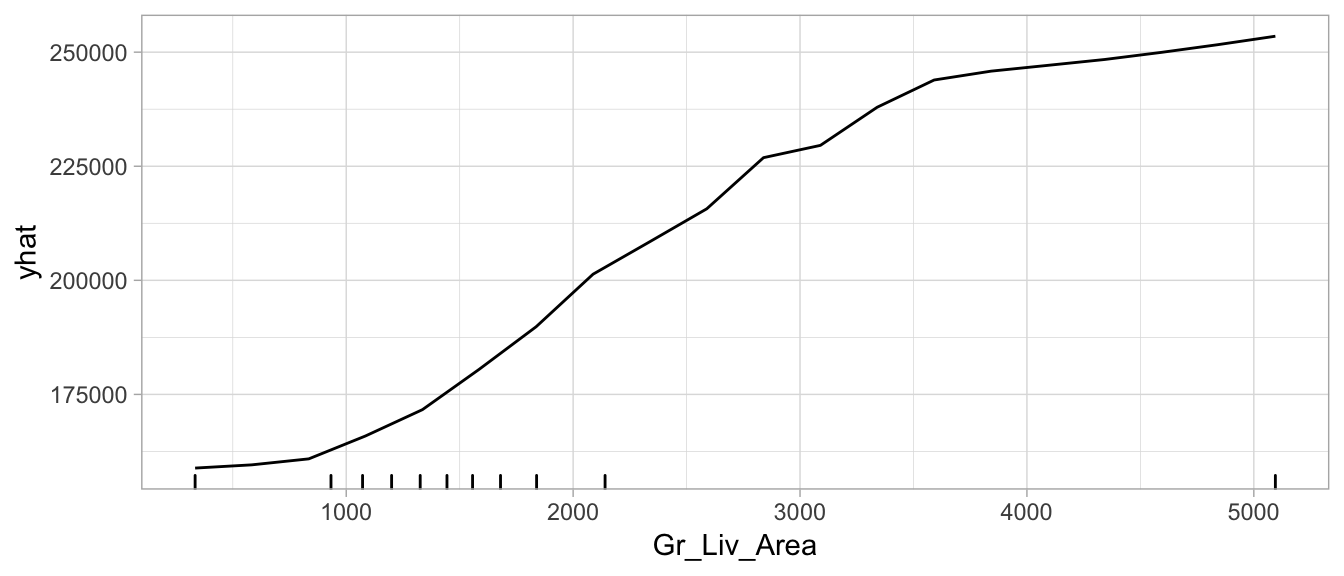
plot(dalex_pdp)
pdp
# Custom prediction function wrapper
pdp_pred <- function(object, newdata)  {
  results <- mean(as.vector(h2o.predict(object, as.h2o(newdata))))
  return(results)
}

# Compute partial dependence values
pd_values <- partial(
  ensemble_tree,
  train = as.data.frame(train_h2o),
  pred.var = "Gr_Liv_Area",
  pred.fun = pdp_pred,
  grid.resolution = 20
)

head(pd_values)
##   Gr_Liv_Area     yhat
## 1         334 158858.2
## 2         584 159566.6
## 3         835 160878.2
## 4        1085 165896.7
## 5        1336 171665.9
## 6        1586 180505.1

autoplot(pd_values,
         rug = TRUE,
         train = as.data.frame(train_h2o))
16.6.3 Adding feature importance
We can assume that those features with larger marginal effects on the response have greater importance, this is really useful to create plots of both feature importance and feature effects.
pd_imp_values <- vip(
  ensemble_tree,
  train = as.data.frame(train_h2o),
  method = "firm",
  feature_names = "Gr_Liv_Area",
  pred.fun = pdp_pred,
  grid.resolution = 20,
  ice = FALSE
)

head(pd_imp_values)