Explaning model’s summary
Let’s explain the summary of a trained model.
mars1 <-
  earth(Sale_Price ~ ., data = ames_train)

mars1
## Selected 41 of 45 terms, and 29 of 308 predictors
## Termination condition: RSq changed by less than 0.001 at 45 terms
## Importance: Gr_Liv_Area, Year_Built, Total_Bsmt_SF, ...
## Number of terms at each degree of interaction: 1 40 (additive model)
## GCV 511589986 RSS 967008439675 GRSq 0.9207836 RSq 0.9268516- The number of terms correspond to the number of coefficients used by the model.
coef(mars1) |> length()## [1] 41summary(mars1)$coefficients |> head(7)## Sale_Price
## (Intercept) 227597.23167
## h(Gr_Liv_Area-3194) -287.99337
## h(3194-Gr_Liv_Area) -58.61227
## h(Year_Built-2002) 3128.13737
## h(2002-Year_Built) -450.63697
## h(Total_Bsmt_SF-2223) -653.13097
## h(2223-Total_Bsmt_SF) -29.03002- The number of predictors is counted after transforming all factors into dummy variables.
recipe(Sale_Price ~ ., data = ames_train) |>
  step_dummy(all_nominal_predictors()) |>
  prep(training = ames_train) |>
  bake(new_data = NULL) |>
  select(-Sale_Price) |>
  ncol()
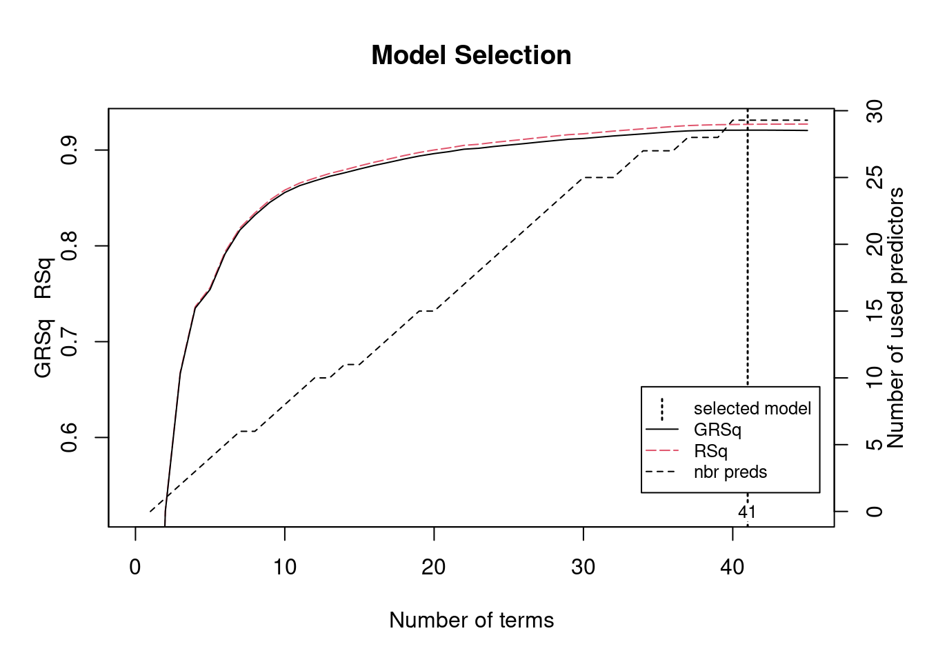
## [1] 308- Shows the path used by
earthto select the model with different metrics
plot(mars1, which = 1)
It’s also important to point out that this package has the capacity to assess potential interactions between different hinge functions.
earth(Sale_Price ~ .,
      data = ames_train,
      degree = 2) |>
  summary() |>
  (\(x) x$coefficients)() |>
  head(10)
## Sale_Price
## (Intercept) 3.473694e+05
## h(Gr_Liv_Area-3194) 2.302940e+02
## h(3194-Gr_Liv_Area) -7.005261e+01
## h(Year_Built-2002) 5.242461e+03
## h(2002-Year_Built) -7.360079e+02
## h(Total_Bsmt_SF-2223) 1.181093e+02
## h(2223-Total_Bsmt_SF) -4.901140e+01
## h(Year_Built-2002)*h(Gr_Liv_Area-2398) 9.035037e+00
## h(Year_Built-2002)*h(2398-Gr_Liv_Area) -3.382639e+00
## h(Bsmt_Unf_SF-625)*h(3194-Gr_Liv_Area) -1.145129e-02