12.3 Vector autoregressions (VAR)
A Bi-directional relationship between response and predictors, such as in case of an increase in income \(I_t\) leading to an increase in consumption \(C_t\) and viceversa, is when every variable is assumed to influence every other variable in the system.
An example of such a situation occurred in Australia during the Global Financial Crisis of 2008–2009. The Australian government issued stimulus packages that included cash payments in December 2008, just in time for Christmas spending. As a result, retailers reported strong sales and the economy was stimulated. Consequently, incomes increased.
A VAR model is a generalisation of the univariate autoregressive model for forecasting a vector of time series.
Variables are endogenous:
\[Y=y_{1,t},y_{2,t},...,y_{s,t}\] \[y_{1,t}=c_1+\phi y_{1,t-1}+ \phi y_{2,t-1}+...+\epsilon_{1,t}\]
Forecasts are generated from a VAR in a recursive manner.
- how many variables (K)
- how many lags (p)
A direct interpretation of the estimated coefficients is difficult.
N. Coefficients:
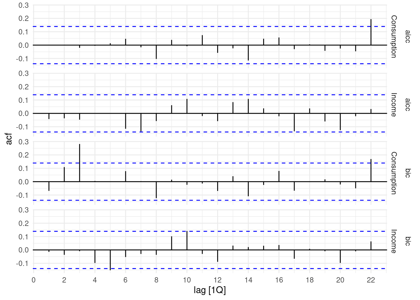
\[K+pK^2\] In VAR models often use the BIC instead of AIC.
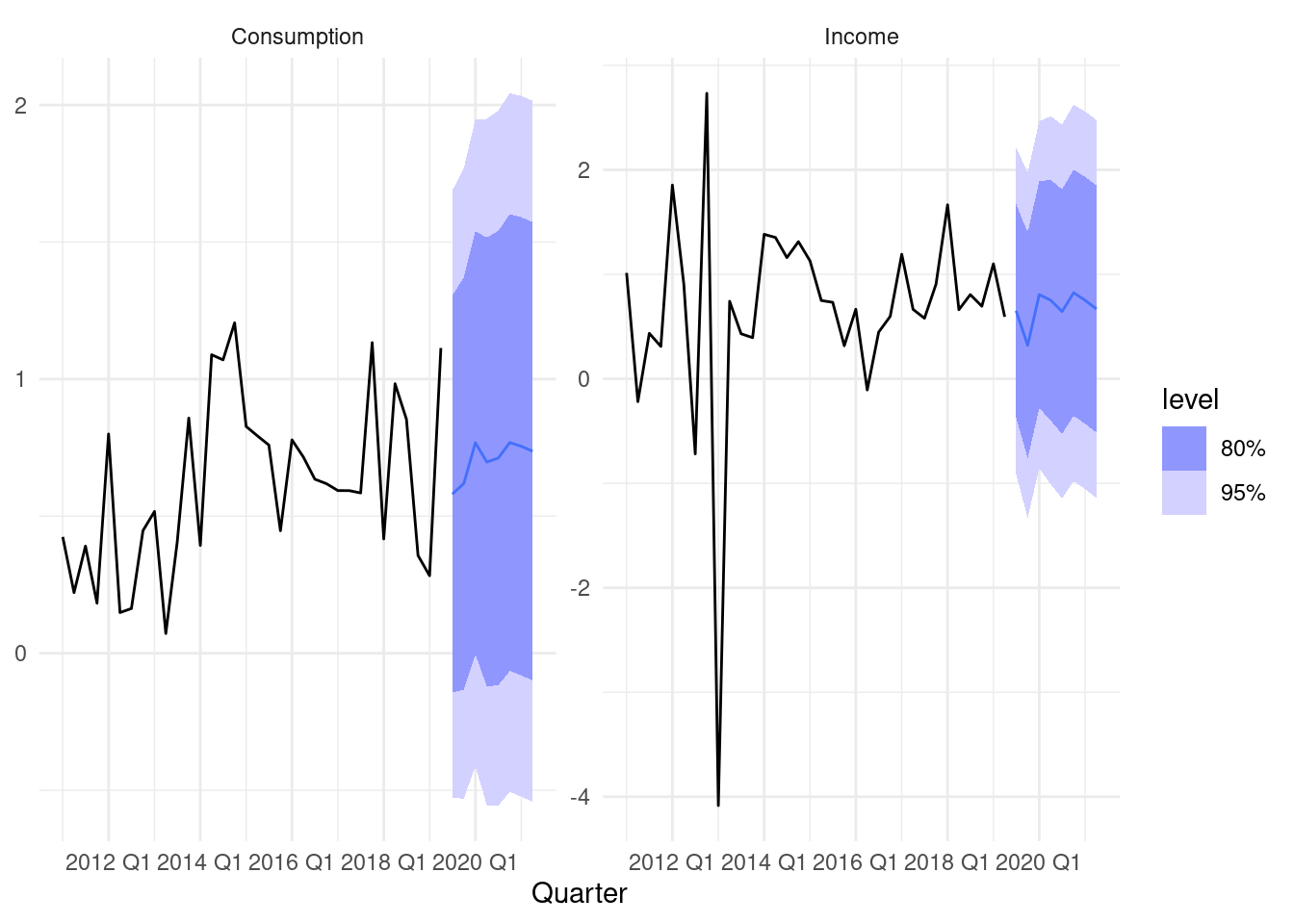
12.3.1 Case Study 5
Forecasting US consumption:
fit5 <- us_change |>
  model(
    aicc = VAR(vars(Consumption, Income)),
    bic = VAR(vars(Consumption, Income), ic = "bic")
  )
fit5
## # A mable: 1 x 2
## aicc bic
## <model> <model>
## 1 <VAR(5) w/ mean> <VAR(1) w/ mean>## # A tibble: 2 × 6
## .model sigma2 log_lik AIC AICc BIC
## <chr> <list> <dbl> <dbl> <dbl> <dbl>
## 1 aicc <dbl [2 × 2]> -373. 798. 806. 883.
## 2 bic <dbl [2 × 2]> -408. 836. 837. 869.