3.3 Classical decompositions

A classical decomposition method is the moving average method to estimate the trend-cycle. It originated in the 1920s and was widely used until the 1950s.

3.3.1 Moving average smoothing

A moving average of order m: seasonal period

$$m=2k+1$$

composed of seasonal patterns estimated based on k consecutive seasonal cycles, where $k$ controls how rapidly the component can change.

The estimate of the trend-cycle at time $t$ is obtained by averaging values of the time series within $k$ periods of $t$.

the average eliminates some of the randomness

$$\hat{T_t}=\frac{1}{m}\sum_{j=-k}^k{y_{t+j}}$$

aus_exports <- global_economy %>%
  filter(Country == "Australia")%>%
   mutate(`3-MA` = slider::slide_dbl(Exports, mean,
                                     .before = 1, # this is k
                                     .after = 1, 
                                     .complete = TRUE),
          `5-MA` = slider::slide_dbl(Exports, mean,
                                     .before = 2, # this is k
                                     .after = 2, 
                                     .complete = TRUE),
          `7-MA` = slider::slide_dbl(Exports, mean,
                                     .before = 3, # this is k
                                     .after = 3, 
                                     .complete = TRUE),
          `9-MA` = slider::slide_dbl(Exports, mean,
                                     .before = 4, # this is k
                                     .after = 4, 
                                     .complete = TRUE)
          ) %>%
  select(Year,Exports,`3-MA`,`5-MA`,`7-MA`,`9-MA`)%>%
  pivot_longer(cols = ends_with("MA"),names_to = "kma",values_to="values")

aus_exports %>% head

## # A tsibble: 6 x 4 [1Y]
## # Key:       kma [4]
##    Year Exports kma   values
##   <dbl>   <dbl> <chr>  <dbl>
## 1  1960    13.0 3-MA    NA  
## 2  1960    13.0 5-MA    NA  
## 3  1960    13.0 7-MA    NA  
## 4  1960    13.0 9-MA    NA  
## 5  1961    12.4 3-MA    13.1
## 6  1961    12.4 5-MA    NA

aus_exports %>%
  autoplot(Exports,color="darkred",size=0.2) +
  geom_line(aes(y = values,color=kma)) +
  labs(y = "% of GDP",x="Year",
       title = "Total Australian exports") +
  guides(colour = guide_legend(title = "series"))+
  ggthemes::scale_color_pander()+
  ggthemes::theme_pander()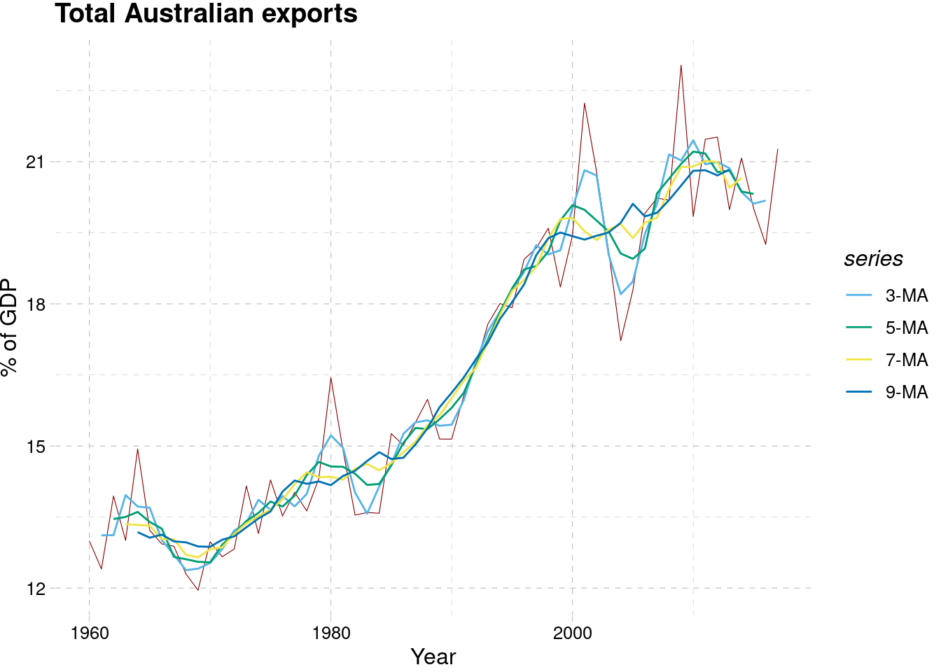

3.3.2 Moving averages of moving averages

When 2-MA follows a moving average of an even order (such as 4), it is called a “centered moving average of order 4”

The most common use of centred moving averages is for estimating the trend-cycle from seasonal data.

beer_ma <- aus_production %>%
  filter(year(Quarter) >= 1992) %>%
  select(Quarter, Beer) %>%
  mutate(`4-MA` = slider::slide_dbl(Beer, mean,
                .before = 1, .after = 2, .complete = TRUE),
         `2x4-MA` = slider::slide_dbl(`4-MA`, mean,
                .before = 1, .after = 0, .complete = TRUE)
  )

beer_ma %>%head

## # A tsibble: 6 x 4 [1Q]
##   Quarter  Beer `4-MA` `2x4-MA`
##     <qtr> <dbl>  <dbl>    <dbl>
## 1 1992 Q1   443    NA       NA 
## 2 1992 Q2   410   451.      NA 
## 3 1992 Q3   420   449.     450 
## 4 1992 Q4   532   452.     450.
## 5 1993 Q1   433   449      450.
## 6 1993 Q2   421   444      446.

3.3.3 Weighted moving averages

Combinations of moving averages result in weighted moving averages.

Weights: $a_k=[\frac{1}{8},\frac{1}{4},\frac{1}{4},\frac{1}{4},\frac{1}{8}]$

k: $k=(m-1)/2$

$$\hat{T_t}=\sum_{j=-k}^k{a_jy_{t+j}}$$

3.3.4 Additive decomposition

In additive decomposition, it is assumed that the seasonal component is constant from year to year.

1. $$m=\left\{\begin{matrix} 2\times m-MA & \text{if m is even}\\ m-MA & \text{if m is odd} \end{matrix}\right.$$

2. De-trend: $y_t-\hat{T_t}$

3. Adjust to ensure that they add to zero

4. $R_t=y_t-\hat{T_t}-\hat{S_t}$

Formula:

?classical_decomposition
model(classical_decomposition(<variable>, type = "additive"))

3.3.5 Multiplicative decomposition

For multiplicative seasonality, the $m$ values that form the seasonal component are sometimes called the “seasonal indices”.

1. $$m=\left\{\begin{matrix} 2\times m-MA & \text{if m is even}\\ m-MA & \text{if m is odd} \end{matrix}\right.$$

2. De-trend: $y_t/\hat{T_t}$

3. Adjust to ensure that they add to zero

4. $R_t=y_t/(\hat{T_t}\hat{S_t})$