9.1 Exercise 7
Consider aus_airpassengers, the total number of passengers (in millions) from Australian air carriers for the period 1970-2011.
# load packages
suppressMessages(library(tidyverse))
library(fpp3)
library(plotly)
theme_set(theme_minimal())## # A tsibble: 6 x 2 [1Y]
## Year Passengers
## <dbl> <dbl>
## 1 1970 7.32
## 2 1971 7.33
## 3 1972 7.80
## 4 1973 9.38
## 5 1974 10.7
## 6 1975 11.1# plot time series
aus_airpassengers %>%
autoplot(Passengers) +
geom_smooth(method = 'loess', se = FALSE, color = 'steelblue') +
labs(title = 'Australia Total Number of Passengers (millions)')## `geom_smooth()` using formula = 'y ~ x'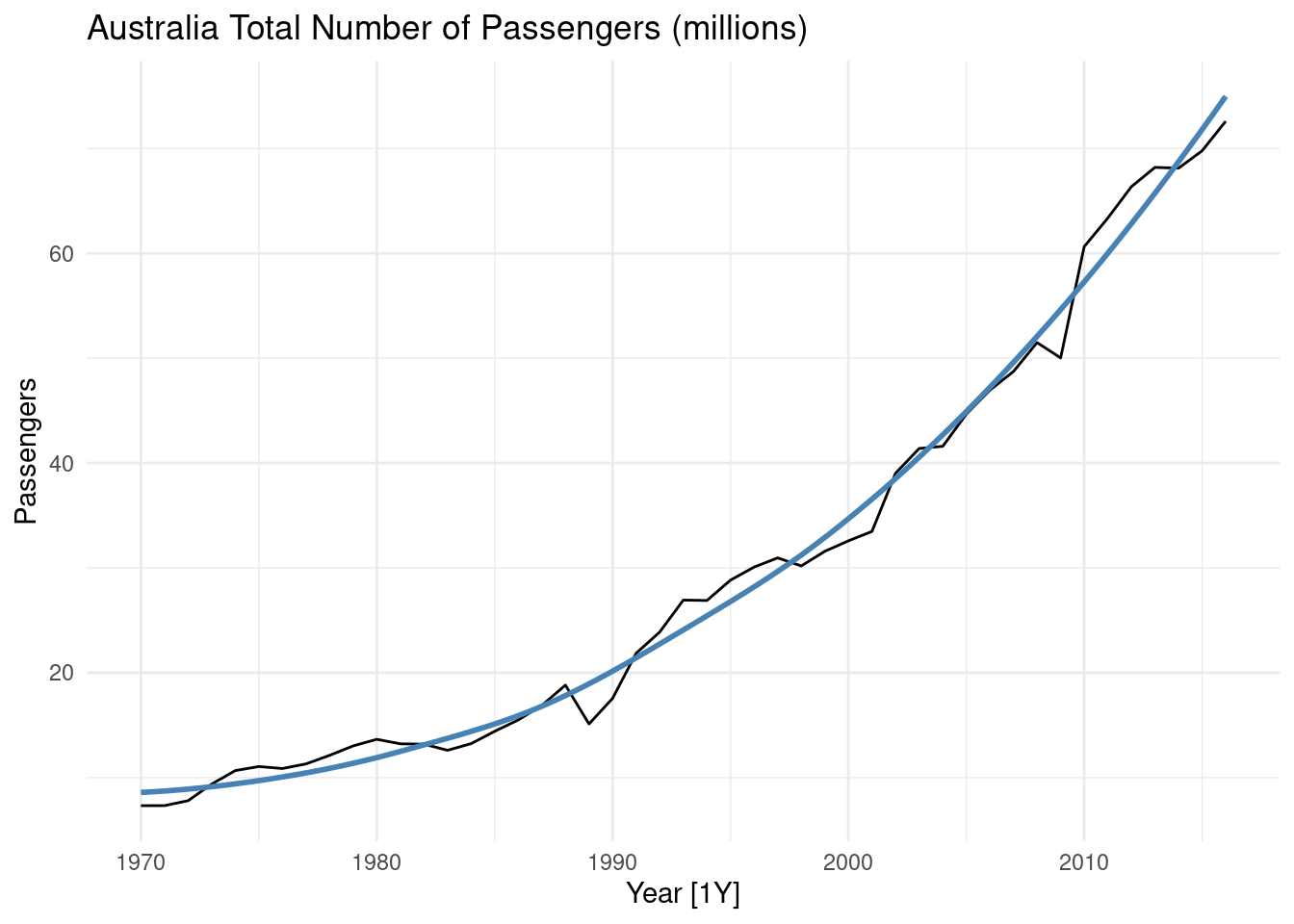
## # A tibble: 1 × 2
##   kpss_stat kpss_pvalue
##       <dbl>       <dbl>
## 1      1.19        0.01
# differencing time series
aus_airpassengers %>%
mutate(Passengers = Passengers %>%
difference(1) %>%
difference(1)) %>%
autoplot(Passengers) +
labs(title = 'Australia Total Number of Passengers (change)')## Warning: Removed 2 rows containing missing values or values outside the scale range
## (`geom_line()`).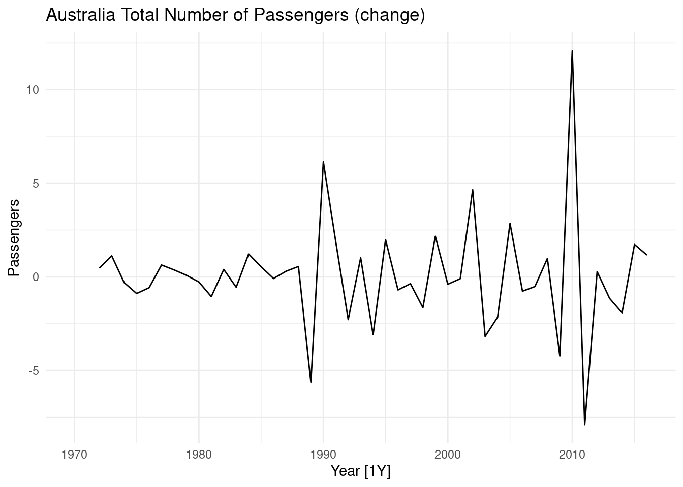
aus_airpassengers %>%
  mutate(Passengers = Passengers %>%
           difference(1) %>%
           difference(1)
  ) %>%
  features(Passengers, unitroot_kpss)
## # A tibble: 1 × 2
## kpss_stat kpss_pvalue
## <dbl> <dbl>
## 1 0.0361 0.19.1.1 a. Use ARIMA() to find an appropriate ARIMA model. What model was selected.
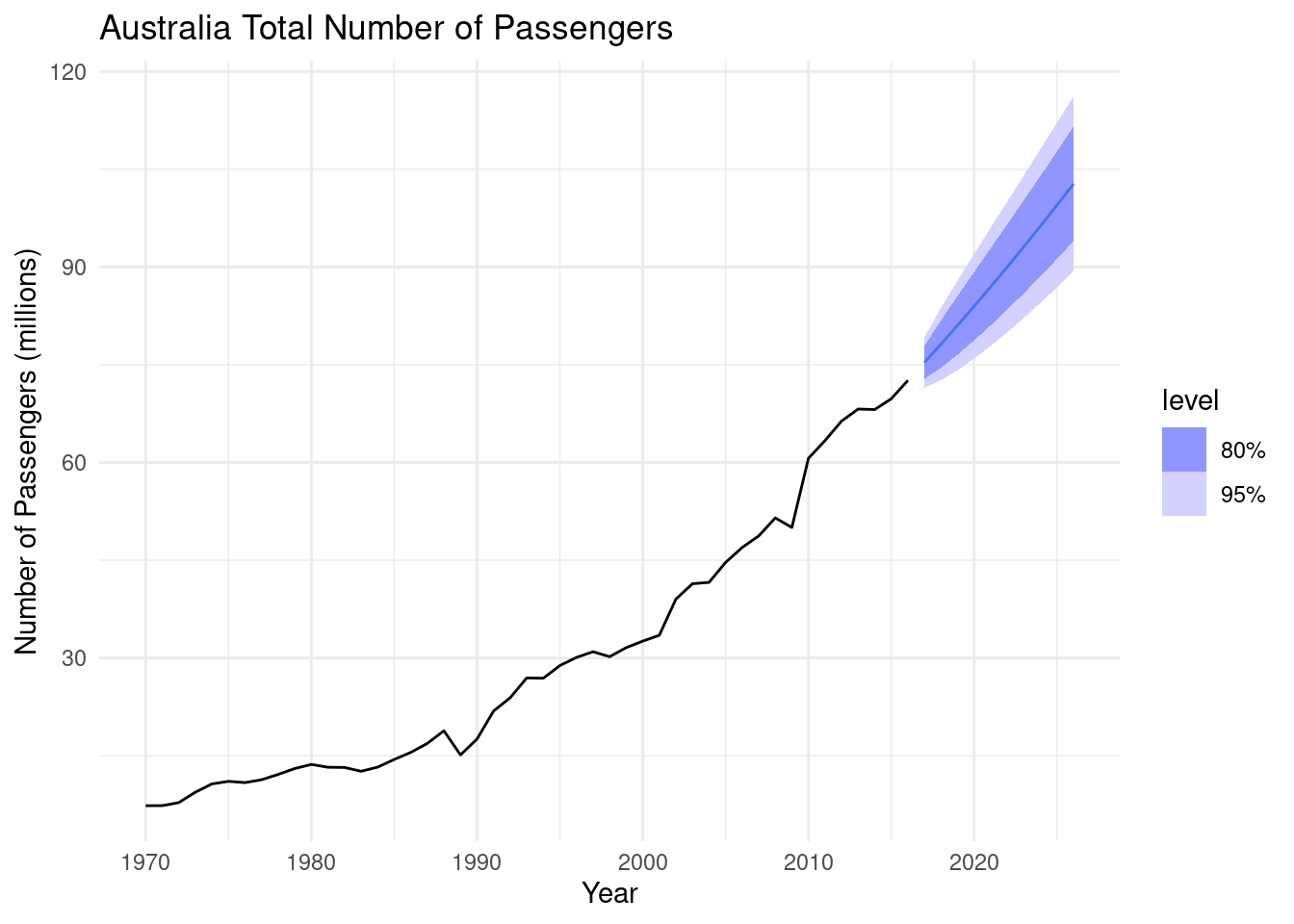
Check that the residuals look like white noise. Plot forecasts for the next 10 periods.
## Series: Passengers
## Model: ARIMA(0,2,1)
##
## Coefficients:
##           ma1
##       -0.8963
## s.e.   0.0594
##
## sigma^2 estimated as 4.308:  log likelihood=-97.02
## AIC=198.04 AICc=198.32 BIC=201.65## # A tibble: 1 × 6
## .model term estimate std.error statistic p.value
## <chr> <chr> <dbl> <dbl> <dbl> <dbl>
## 1 ARIMA(Passengers) ma1 -0.896 0.0594 -15.1 3.24e-19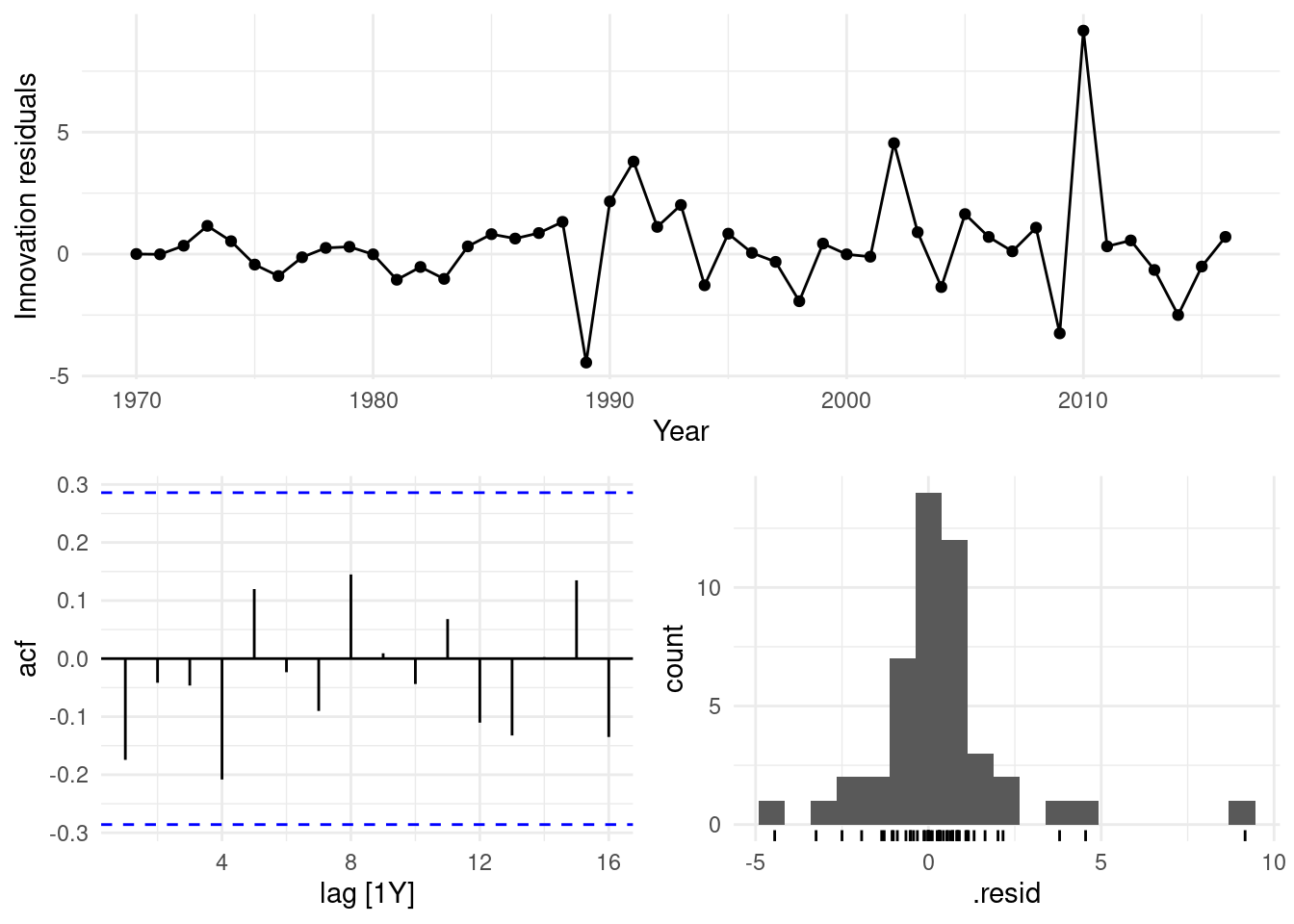
# forecasts for the next 10 years (periods)
fit_1 |> forecast(h=10) |>
  autoplot(aus_airpassengers) +
  labs(y = "Number of Passengers (millions)",
       title = "Australia Total Number of Passengers")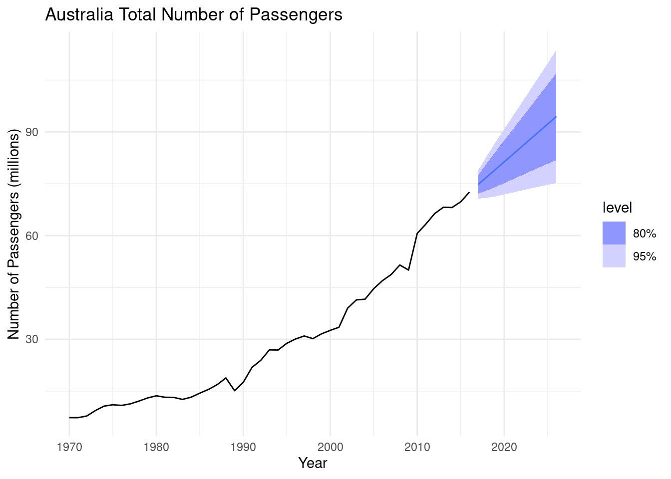
9.1.3 c. Plot forecasts from an ARIMA(0,1,0) model with drift and compare these to part a.
## Series: Passengers
## Model: ARIMA(0,1,0) w/ drift
##
## Coefficients:
##       constant
##         1.4191
## s.e.    0.3014
##
## sigma^2 estimated as 4.271:  log likelihood=-98.16
## AIC=200.31 AICc=200.59 BIC=203.97## # A tibble: 1 × 6
## .model term estimate std.error statistic p.value
## <chr> <chr> <dbl> <dbl> <dbl> <dbl>
## 1 ARIMA(Passengers ~ 1 + pdq(0, 1, 0… cons… 1.42 0.301 4.71 2.32e-5# plot forecasts (h = 10)
fit_2 |> forecast(h=10) |>
autoplot(aus_airpassengers) +
labs(y = "Number of Passengers (millions)",
title = "Australia Total Number of Passengers")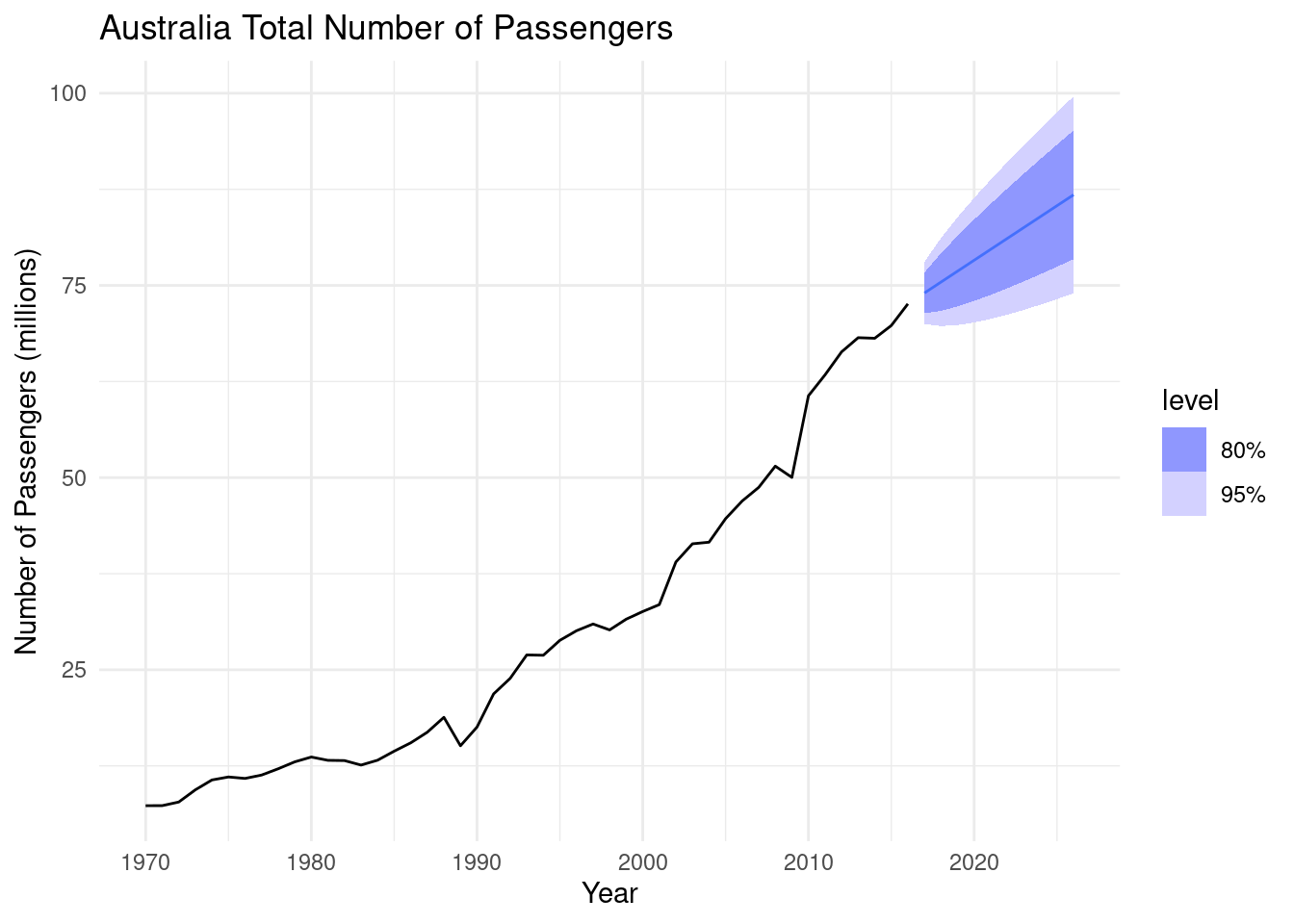
9.1.4 d. Plot forecasts from an ARIMA(2,1,2) model with drift and compare these to parts a. and c.
Remove the constant and see what happens.
## Series: Passengers
## Model: ARIMA(2,1,2) w/ drift
##
## Coefficients:
##           ar1      ar2     ma1     ma2  constant
##       -0.5518  -0.7327  0.5895  1.0000    3.2216
## s.e.   0.1684   0.1224  0.0916  0.1008    0.7224
##
## sigma^2 estimated as 4.031:  log likelihood=-96.23
## AIC=204.46 AICc=206.61 BIC=215.43## # A tibble: 5 × 6
## .model term estimate std.error statistic p.value
## <chr> <chr> <dbl> <dbl> <dbl> <dbl>
## 1 ARIMA(Passengers ~ 1 + pdq(2, 1, … ar1 -0.552 0.168 -3.28 2.00e- 3
## 2 ARIMA(Passengers ~ 1 + pdq(2, 1, … ar2 -0.733 0.122 -5.99 3.03e- 7
## 3 ARIMA(Passengers ~ 1 + pdq(2, 1, … ma1 0.589 0.0916 6.43 6.45e- 8
## 4 ARIMA(Passengers ~ 1 + pdq(2, 1, … ma2 1.00 0.101 9.92 5.18e-13
## 5 ARIMA(Passengers ~ 1 + pdq(2, 1, … cons… 3.22 0.722 4.46 5.26e- 5# plot forecasts (h = 10)
fit_3 |> forecast(h=10) |>
autoplot(aus_airpassengers) +
labs(y = "Number of Passengers (millions)",
title = "Australia Total Number of Passengers")
# Arima without constant
fit_3_constant <- aus_airpassengers %>%
  as.ts() %>%
  forecast::Arima(c(2, 1, 2), include.constant = TRUE)

fit_3_constant
## Series: .
## ARIMA(2,1,2) with drift
##
## Coefficients:
## ar1 ar2 ma1 ma2 drift
## -0.5518 -0.7327 0.5895 1.0000 1.4101
## s.e. 0.1684 0.1224 0.0916 0.1008 0.3162
##
## sigma^2 = 4.031: log likelihood = -96.23
## AIC=204.46 AICc=206.61 BIC=215.43## Series: .
## ARIMA(0,2,1)
##
## Coefficients:
## ma1
## -0.8963
## s.e. 0.0594
##
## sigma^2 = 4.308: log likelihood = -97.02
## AIC=198.04 AICc=198.32 BIC=201.659.1.5 e. Plot forecasts from an ARIMA(0,2,1) model with a constant. What happens?
## Warning: Model specification induces a quadratic or higher order polynomial trend.
## This is generally discouraged, consider removing the constant or reducing the number of differences.## Series: Passengers
## Model: ARIMA(0,2,1) w/ poly
##
## Coefficients:
## ma1 constant
## -1.0000 0.0571
## s.e. 0.0585 0.0213
##
## sigma^2 estimated as 3.855: log likelihood=-95.1
## AIC=196.21 AICc=196.79 BIC=201.63## # A tibble: 2 × 6
## .model term estimate std.error statistic p.value
## <chr> <chr> <dbl> <dbl> <dbl> <dbl>
## 1 ARIMA(Passengers ~ 1 + pdq(0, 2, … ma1 -1.00 0.0585 -17.1 2.70e-21
## 2 ARIMA(Passengers ~ 1 + pdq(0, 2, … cons… 0.0571 0.0213 2.68 1.03e- 2# plot forecasts (h = 10)
fit_4 |> forecast(h=10) |>
autoplot(aus_airpassengers) +
labs(y = "Number of Passengers (millions)",
title = "Australia Total Number of Passengers")