12.4 Neural network models

Example of a multilayer feed-forward network.

Each layer of nodes receives inputs from the previous layers.

The outputs of the nodes in one layer are inputs to the next layer.

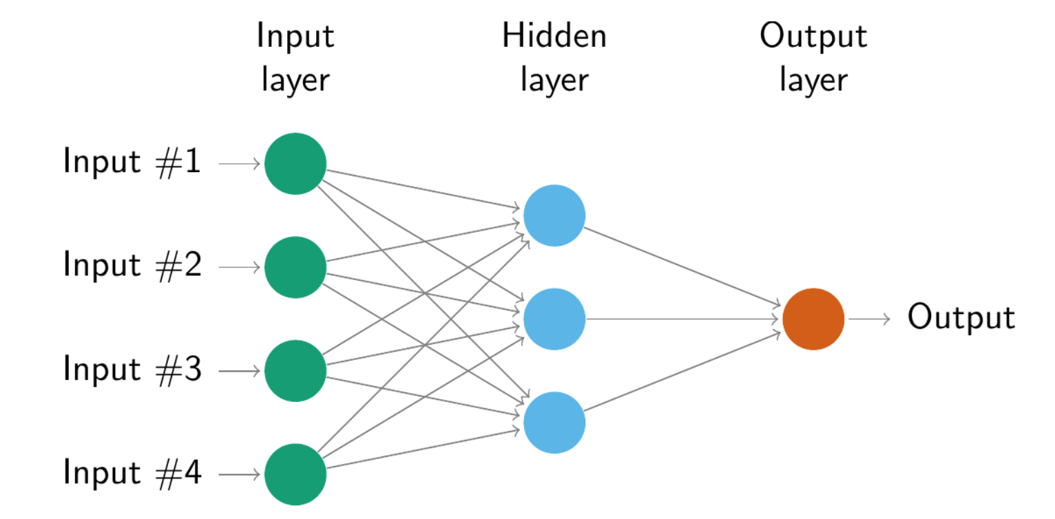
\[z_j=b_j+\sum_{1}^n{w_{i,j}x_{i,j}}\]

\[s(z)=\frac{1}{1+e^{-z}}\] The weights starts with an assigned random value, and then updated using the observed data.

The model is neural network auto-regressive model \(NNAR(p,k)\) where p are lagged inputs and k the nodes in the hidden layer.

\(NNAR(p,0)\) model is equivalent to an \(ARIMA(p,0,0)\) While \(NNAR(p,P,k)_m\) is a model with more layers and it is equivalent to \(ARIMA(p,0,0)(P,0,0)_m\)

The default value for k is \(k=(p+P+1)/2\)

12.4.1 Case Study 6

Sunspots, dark spots on the sun surface, follow a cycle of length between 9 and 14 years.

sunspots <- sunspot.year |> 
  as_tsibble()
sunspots%>%head()

## # A tsibble: 6 x 2 [1Y]
##   index value
##   <dbl> <dbl>
## 1  1700     5
## 2  1701    11
## 3  1702    16
## 4  1703    23
## 5  1704    36
## 6  1705    58

fit6 <- sunspots |>
  model(NNETAR(sqrt(value)))

fit6 %>% gg_tsresiduals()

## Warning: Removed 9 rows containing missing values or values outside the scale range
## (`geom_line()`).

## Warning: Removed 9 rows containing missing values or values outside the scale range
## (`geom_point()`).

## Warning: Removed 9 rows containing non-finite outside the scale range
## (`stat_bin()`).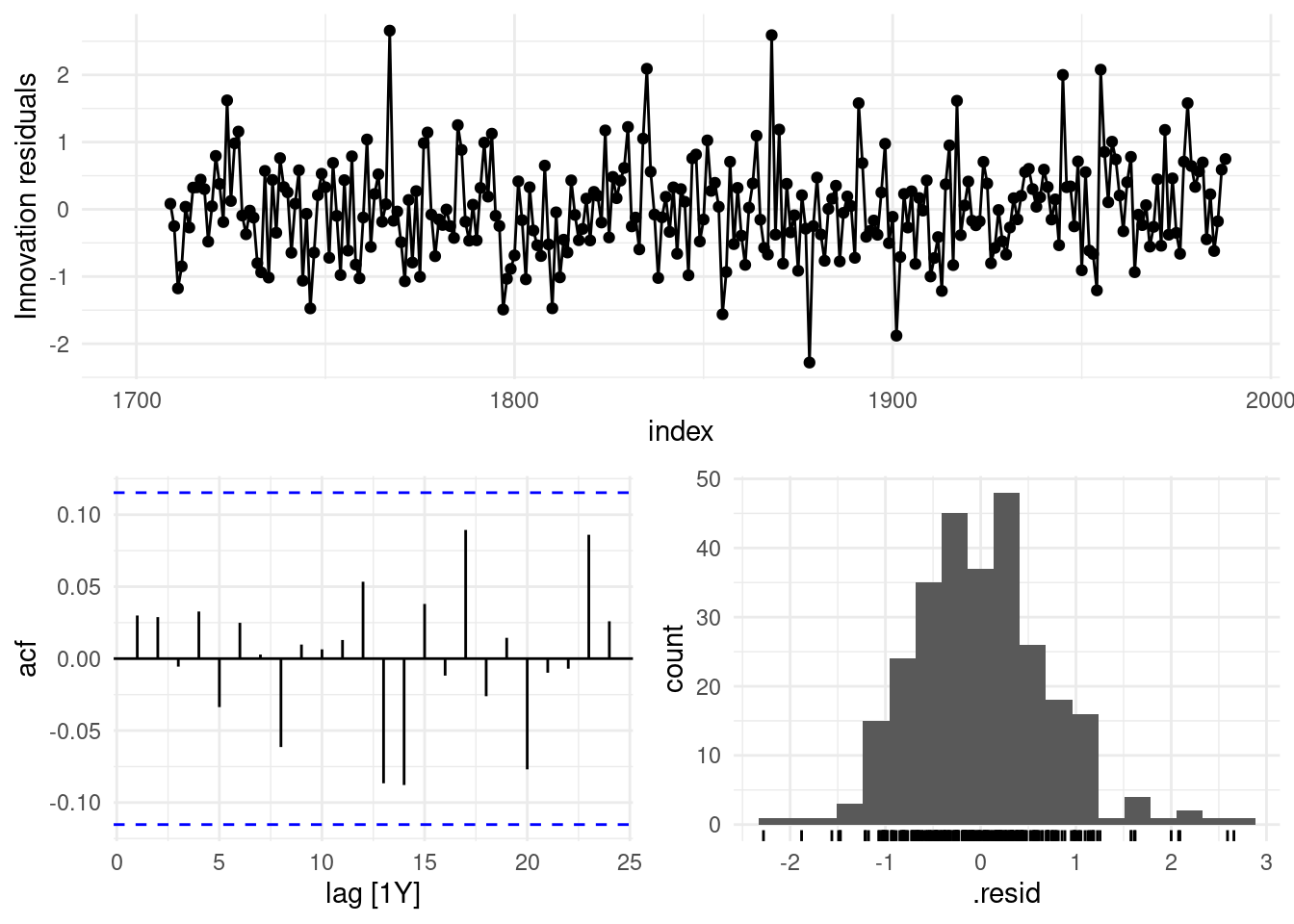

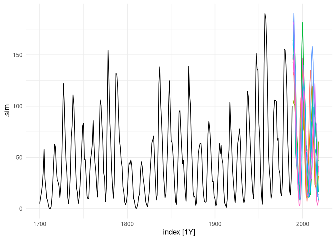
Forecasting neural network time series is an iterative procedure, and might take a while to compile.

pred <- fit6 |>
  forecast(h = 1)

\[y_t=f(y_{t-1},\epsilon_t)\]

12.4.1.1 Bootstrap application

Here is a simulation of 9 possible future sample paths (times = 9), 30 years ahead (h = 30).

fit6 |>
  # bootstrapping
  generate(times = 9, h = 30) |>
  autoplot(.sim) +
  autolayer(sunspots, value) +
  theme(legend.position = "none")