8.3 Exercises

8.3.1 Exercise 5

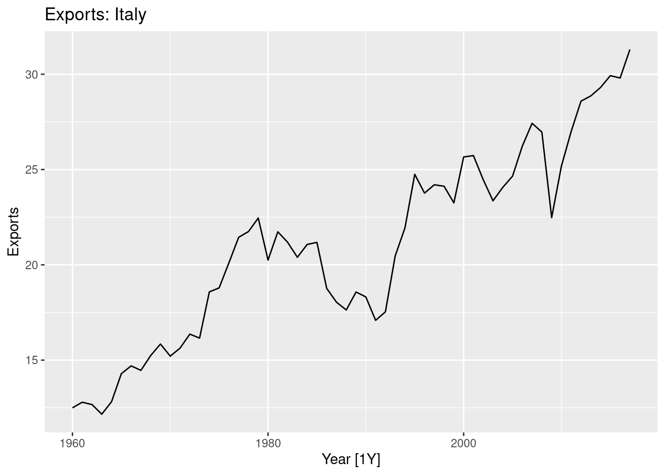
Data set global_economy contains the annual Exports from many countries.

8.3.1.1 Select one country to analyse.

library(fpp3)
italy_economy <- global_economy %>%
  filter(Country=="Italy")

italy_economy %>% head

## # A tsibble: 6 x 9 [1Y]
## # Key:       Country [1]
##   Country Code   Year          GDP Growth   CPI Imports Exports Population
##   <fct>   <fct> <dbl>        <dbl>  <dbl> <dbl>   <dbl>   <dbl>      <dbl>
## 1 Italy   ITA    1960 40385288344.  NA     4.15    12.9    12.5   50199700
## 2 Italy   ITA    1961 44842760293.   8.21  4.23    12.9    12.8   50536350
## 3 Italy   ITA    1962 50383891899.   6.20  4.43    13.2    12.7   50879450
## 4 Italy   ITA    1963 57710743060.   5.61  4.76    14.3    12.2   51252000
## 5 Italy   ITA    1964 63175417019.   2.80  5.04    12.7    12.8   51675350
## 6 Italy   ITA    1965 67978153851.   3.27  5.27    12.1    14.3   52112350

8.3.1.2 Plot the Exports series and discuss the main features of the data.

italy_economy |>
  autoplot(Exports) +
  labs(y = "Exports", title = "Exports: Italy")

italy_economy%>%
  tail()

## # A tsibble: 6 x 9 [1Y]
## # Key:       Country [1]
##   Country Code   Year     GDP Growth   CPI Imports Exports Population
##   <fct>   <fct> <dbl>   <dbl>  <dbl> <dbl>   <dbl>   <dbl>      <dbl>
## 1 Italy   ITA    2012 2.07e12 -2.82   106.    27.6    28.6   59539717
## 2 Italy   ITA    2013 2.13e12 -1.73   107.    26.6    28.9   60233948
## 3 Italy   ITA    2014 2.15e12  0.114  107.    26.5    29.3   60789140
## 4 Italy   ITA    2015 1.83e12  0.952  107.    27.0    29.9   60730582
## 5 Italy   ITA    2016 1.86e12  0.858  107.    26.5    29.8   60627498
## 6 Italy   ITA    2017 1.93e12  1.50   109.    28.2    31.3   60551416

8.3.1.3 Use an ETS(A,N,N) model to forecast the series, and plot the forecasts.

# Estimate parameters
fit <- italy_economy |>
  model(ETS(Exports ~ error("A") + trend("N") + season("N")))
fit %>% tidy()

## # A tibble: 2 × 4
##   Country .model                                                  term  estimate
##   <fct>   <chr>                                                   <chr>    <dbl>
## 1 Italy   "ETS(Exports ~ error(\"A\") + trend(\"N\") + season(\"… alpha     1.00
## 2 Italy   "ETS(Exports ~ error(\"A\") + trend(\"N\") + season(\"… l[0]     12.5

fc <- fit |>
  forecast(h = 5)

fc |>
  autoplot(italy_economy) +
  geom_line(aes(y = .fitted), col="purple",
            data = augment(fit)) +
  labs(y="Exports", title="Exports: Italy") +
  guides(colour = "none")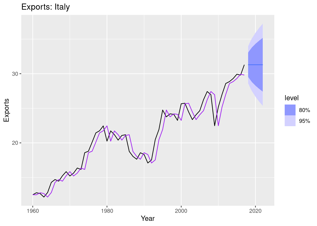

8.3.1.4 Compute the RMSE values for the training data.

italy_economy %>%
  as_tsibble() 

## # A tsibble: 58 x 9 [1Y]
## # Key:       Country [1]
##    Country Code   Year          GDP Growth   CPI Imports Exports Population
##    <fct>   <fct> <dbl>        <dbl>  <dbl> <dbl>   <dbl>   <dbl>      <dbl>
##  1 Italy   ITA    1960 40385288344.  NA     4.15    12.9    12.5   50199700
##  2 Italy   ITA    1961 44842760293.   8.21  4.23    12.9    12.8   50536350
##  3 Italy   ITA    1962 50383891899.   6.20  4.43    13.2    12.7   50879450
##  4 Italy   ITA    1963 57710743060.   5.61  4.76    14.3    12.2   51252000
##  5 Italy   ITA    1964 63175417019.   2.80  5.04    12.7    12.8   51675350
##  6 Italy   ITA    1965 67978153851.   3.27  5.27    12.1    14.3   52112350
##  7 Italy   ITA    1966 73654870011.   5.98  5.39    13.0    14.7   52519000
##  8 Italy   ITA    1967 81133120065.   7.18  5.60    13.5    14.5   52900500
##  9 Italy   ITA    1968 87942231678.   6.54  5.67    13.3    15.2   53235750
## 10 Italy   ITA    1969 97085082807.   6.10  5.82    14.5    15.8   53537950
## # ℹ 48 more rows

italy_economy %>%
  model(ETS(Exports ~ error("A") + trend("N") + season("N"))) |>
    fabletools::accuracy()

## # A tibble: 1 × 11
##   Country .model        .type    ME  RMSE   MAE   MPE  MAPE  MASE RMSSE     ACF1
##   <fct>   <chr>         <chr> <dbl> <dbl> <dbl> <dbl> <dbl> <dbl> <dbl>    <dbl>
## 1 Italy   "ETS(Exports… Trai… 0.324  1.34  1.00  1.39  4.75 0.983 0.991 -0.00701

italy_economy %>%
  as_tsibble() %>% 
  # Perform stretching windows on a tsibble by row
  stretch_tsibble(.init = 10)  |>
  model(ETS(Exports ~ error("A") + trend("N") + season("N"))) |>
    forecast(h = 1) |>
    fabletools::accuracy(italy_economy) 

## Warning: The future dataset is incomplete, incomplete out-of-sample data will be treated as missing. 
## 1 observation is missing at 2018

## # A tibble: 1 × 11
##   .model         Country .type    ME  RMSE   MAE   MPE  MAPE  MASE RMSSE    ACF1
##   <chr>          <fct>   <chr> <dbl> <dbl> <dbl> <dbl> <dbl> <dbl> <dbl>   <dbl>
## 1 "ETS(Exports … Italy   Test  0.321  1.44  1.11  1.20  5.01  1.09  1.07 0.00107

8.3.1.5 Compare the results to those from an ETS(A,A,N) model.

italy_economy %>%
  model(ETS(Exports ~ error("A") + trend("N") + season("N")),
        ETS(Exports ~ error("A") + trend("A") + season("N"))) |>
    fabletools::accuracy()%>%
  select(.model,.type,RMSE)

## # A tibble: 2 × 3
##   .model                                                       .type     RMSE
##   <chr>                                                        <chr>    <dbl>
## 1 "ETS(Exports ~ error(\"A\") + trend(\"N\") + season(\"N\"))" Training  1.34
## 2 "ETS(Exports ~ error(\"A\") + trend(\"A\") + season(\"N\"))" Training  1.30

italy_economy |>
  as_tsibble() |>
  # Perform stretching windows on a tsibble by row
  stretch_tsibble(.init = 10)  |>
  model(SES = ETS(Exports ~ error("A") + trend("N") + season("N")),
        Holt = ETS(Exports ~ error("A") + trend("A") + season("N")),
        Damped = ETS(Exports ~ error("A") + trend("Ad") + season("N")))|>
    forecast(h = 1) |>
    fabletools::accuracy(italy_economy) 

## Warning: The future dataset is incomplete, incomplete out-of-sample data will be treated as missing. 
## 1 observation is missing at 2018

## # A tibble: 3 × 11
##   .model Country .type     ME  RMSE   MAE    MPE  MAPE  MASE RMSSE    ACF1
##   <chr>  <fct>   <chr>  <dbl> <dbl> <dbl>  <dbl> <dbl> <dbl> <dbl>   <dbl>
## 1 Damped Italy   Test  0.144   1.51  1.14 0.411   5.17  1.12  1.12 0.0800 
## 2 Holt   Italy   Test  0.0562  1.52  1.15 0.0414  5.26  1.13  1.13 0.0566 
## 3 SES    Italy   Test  0.321   1.44  1.11 1.20    5.01  1.09  1.07 0.00107

(Remember that the trended model is using one more parameter than the simpler model.)

Discuss the merits of the two forecasting methods for this data set.

8.3.1.6 Compare the forecasts from both methods.

Which do you think is best?

fit <- italy_economy |>
  model(
    SES = ETS(Exports ~ error("A") + trend("N") + season("N")),
    Holt = ETS(Exports ~ error("A") + trend("A") + season("N"))
  )
fc <- fit |> forecast(h = "3 years")


fc |>
  autoplot(italy_economy, level = NULL) +
  labs(title="Italian Exports",
       y="Exports") +
  guides(colour = guide_legend(title = "Forecast"))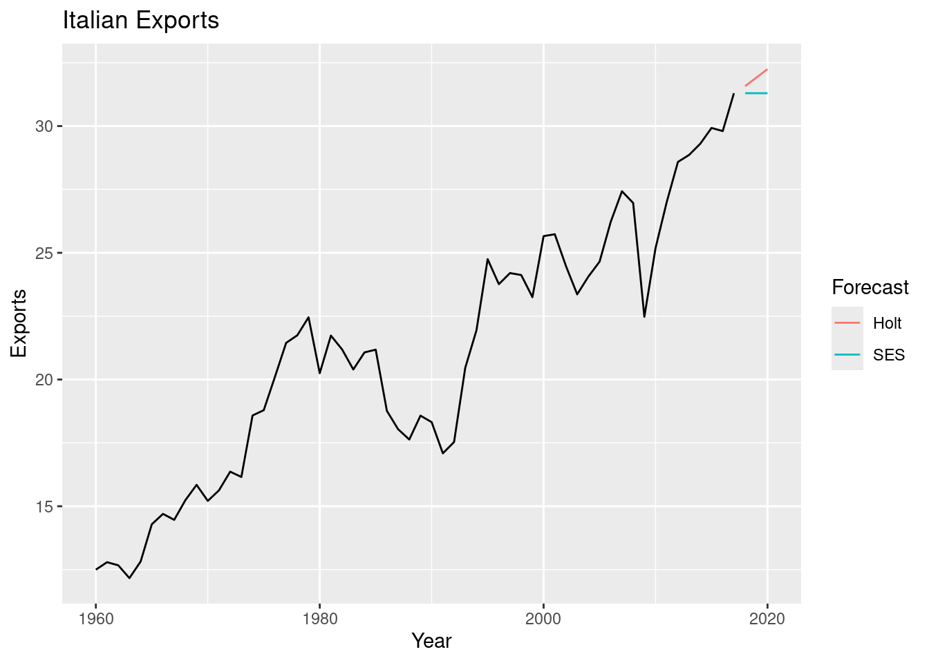

italy_economy |>
  model(
    SES = ETS(Exports ~ error("A") + trend("N") + season("N")),
    Holt = ETS(Exports ~ error("A") + trend("A") + season("N"))
  ) |>
  forecast(h = 15) |>
  autoplot(italy_economy, level = NULL) +
  labs(title = "Italian Exports",
       y = "Exports") +
  guides(colour = guide_legend(title = "Forecast"))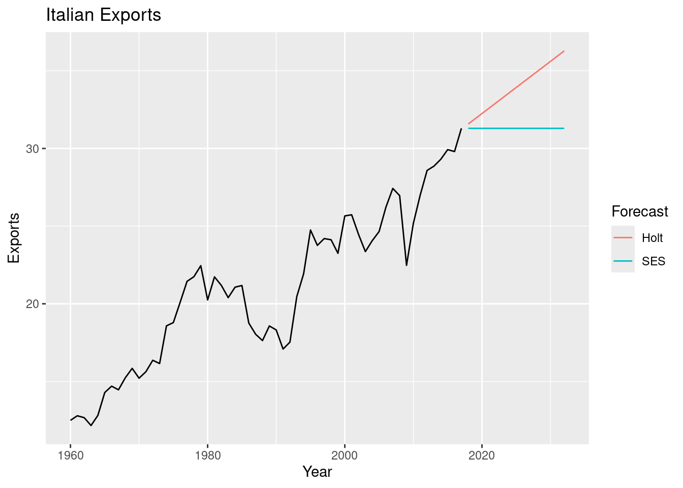

Calculate a 95% prediction interval for the first forecast for each model, using the RMSE values and assuming normal errors.

fit |>
  forecast(h = 1) |>
  autoplot(italy_economy) +
  labs(x="Year", y="Exports",
       title = "Italian Exports")

## Warning in min(x, na.rm = na.rm): no non-missing arguments to min; returning
## Inf

## Warning in max(x, na.rm = na.rm): no non-missing arguments to max; returning
## -Inf

## Warning in min(x, na.rm = na.rm): no non-missing arguments to min; returning
## Inf

## Warning in max(x, na.rm = na.rm): no non-missing arguments to max; returning
## -Inf

## Warning in min(x, na.rm = na.rm): no non-missing arguments to min; returning
## Inf

## Warning in max(x, na.rm = na.rm): no non-missing arguments to max; returning
## -Inf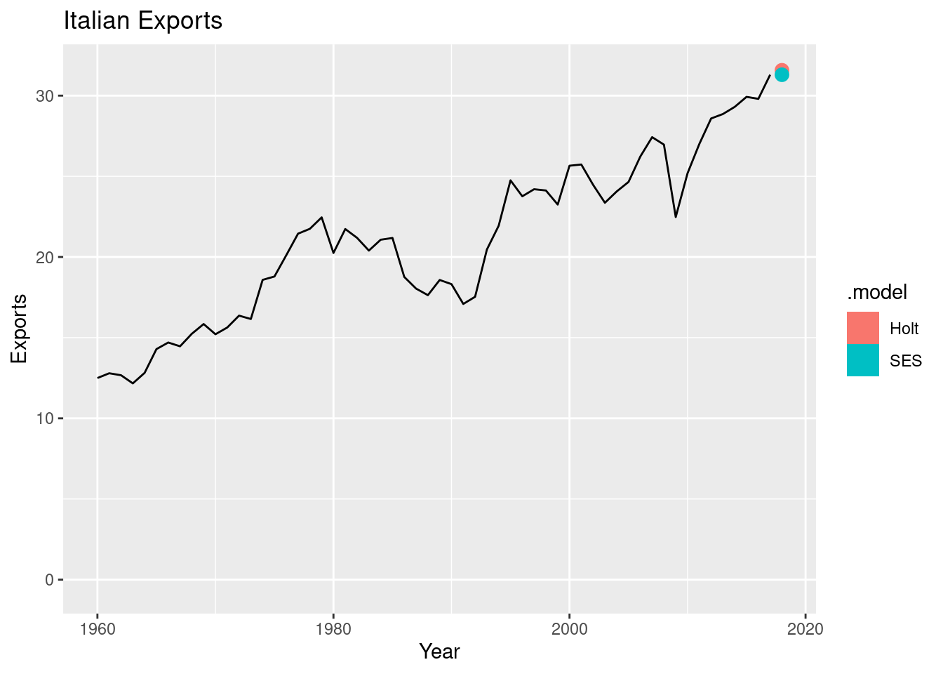

fit |>
  forecast(h = 1)

## # A fable: 2 x 5 [1Y]
## # Key:     Country, .model [2]
##   Country .model  Year    Exports .mean
##   <fct>   <chr>  <dbl>     <dist> <dbl>
## 1 Italy   SES     2018 N(31, 1.8)  31.3
## 2 Italy   Holt    2018 N(32, 1.8)  31.6

Compare your intervals with those produced using R.

Prediction intervals A prediction interval gives an interval within which we expect \(y_t\) to lie with a specified probability. For example, assuming that distribution of future observations is normal, a 95% prediction interval for the \(h\) step forecast is:

\[\hat{y}_{T+h|T} \pm 1.96 \hat{\sigma}_h\]

italy_economy |>
  model(
    SES = ETS(Exports ~ error("A") + trend("N") + season("N")),
    Holt = ETS(Exports ~ error("A") + trend("A") + season("N"))
  ) |>
  forecast(h = 1) |>
  hilo()

## # A tsibble: 2 x 7 [1Y]
## # Key:       Country, .model [2]
##   Country .model  Year    Exports .mean                  `80%`
##   <fct>   <chr>  <dbl>     <dist> <dbl>                 <hilo>
## 1 Italy   SES     2018 N(31, 1.8)  31.3 [29.55514, 33.03762]80
## 2 Italy   Holt    2018 N(32, 1.8)  31.6 [29.85396, 33.29475]80
## # ℹ 1 more variable: `95%` <hilo>