Exercises
- Data is from
vic_elec Australia January 2014 electricity demand and maximum temperatures.
jan14_vic_elec <- vic_elec |>
  filter(yearmonth(Time) == yearmonth("2014 Jan")) |>
  tsibble::index_by(Date = as_date(Time)) |>
  summarise(
    Demand = sum(Demand),
    Temperature = max(Temperature)
  )

jan14_vic_elec%>%head
## # A tsibble: 6 x 3 [1D]
##   Date        Demand Temperature
##   <date>       <dbl>       <dbl>
## 1 2014-01-01 175185.        26
## 2 2014-01-02 188351.        23
## 3 2014-01-03 189086.        22.2
## 4 2014-01-04 173798.        20.3
## 5 2014-01-05 169733.        26.1
## 6 2014-01-06 195241.        19.6
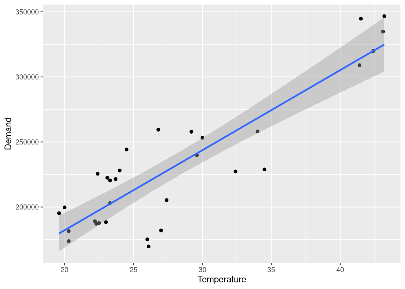
- Plot the data and find the regression model for Demand with temperature as a predictor variable. Why is there a positive relationship?
ggplot(jan14_vic_elec,aes(x=Temperature,y=Demand))+
  geom_point()+
  geom_smooth(method = "lm")
## `geom_smooth()` using formula = 'y ~ x'
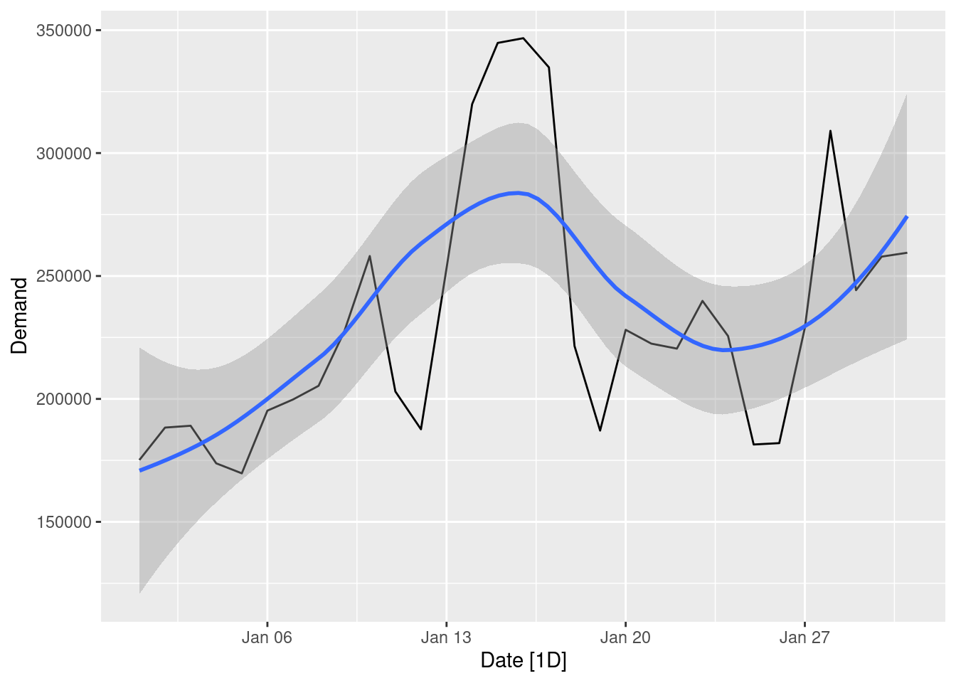
- Produce a residual plot. Is the model adequate? Are there any outliers or influential observations?
jan14_vic_elec%>%
  autoplot()+
  geom_smooth()
## Plot variable not specified, automatically selected `.vars = Demand`
## `geom_smooth()` using method = 'loess' and formula = 'y ~ x'
- Use the model to forecast the electricity demand that you would expect for the next day if the maximum temperature was 15∘C and compare it with the forecast if the with maximum temperature was 35∘C. Do you believe these forecasts? The following R code will get you started:
jan14_vic_elec |>
  model(TSLM(Demand ~ Temperature)) |>
  forecast(
    new_data(jan14_vic_elec, 1) |>
      mutate(Temperature = 15)
  ) |>
  autoplot(jan14_vic_elec)
## Warning: Computation failed in `stat_interval()`.
## Caused by error in `trans$transform()`:
## ! `transform_date()` works with objects of class <Date> only
## Warning in min(x, na.rm = na.rm): no non-missing arguments to min; returning
## Inf
## Warning in max(x, na.rm = na.rm): no non-missing arguments to max; returning
## -Inf
## Warning in min(x, na.rm = na.rm): no non-missing arguments to min; returning
## Inf
## Warning in max(x, na.rm = na.rm): no non-missing arguments to max; returning
## -Inf
## Warning in min(x, na.rm = na.rm): no non-missing arguments to min; returning
## Inf
## Warning in max(x, na.rm = na.rm): no non-missing arguments to max; returning
## -Inf
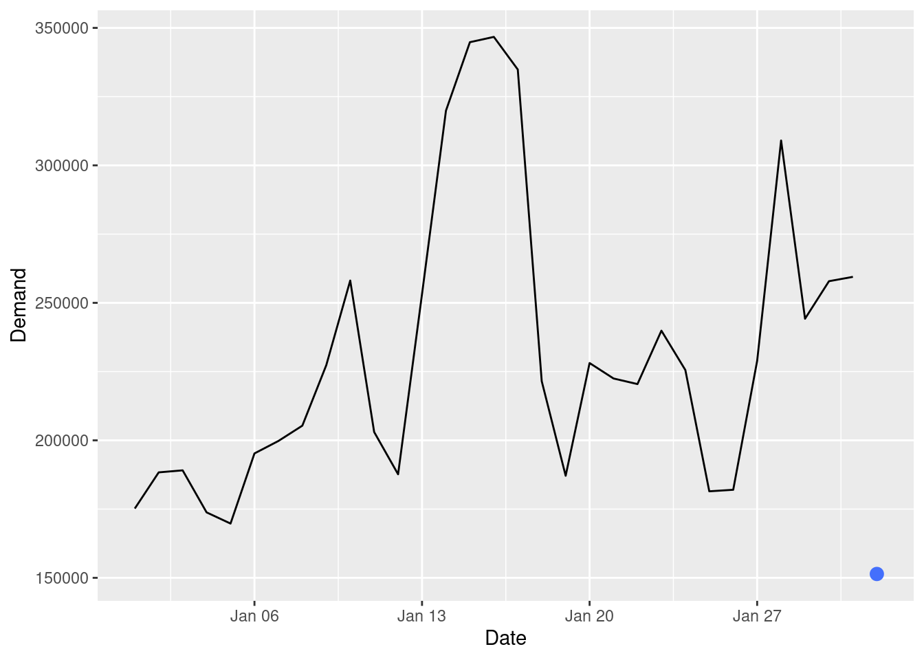
fcst_vic_elec_jan14_15 <- jan14_vic_elec %>%
     model(tslm = TSLM(Demand ~ Temperature)) %>%
     forecast(
          new_data(jan14_vic_elec, 1) %>%
               mutate(Temperature = 15)
     )

fcst_vic_elec_jan14_15 %>%
     autoplot()
## Warning: Computation failed in `stat_interval()`.
## Caused by error in `trans$transform()`:
## ! `transform_date()` works with objects of class <Date> only
## Warning in min(x, na.rm = na.rm): no non-missing arguments to min; returning
## Inf
## Warning in max(x, na.rm = na.rm): no non-missing arguments to max; returning
## -Inf
## Warning in min(x, na.rm = na.rm): no non-missing arguments to min; returning
## Inf
## Warning in max(x, na.rm = na.rm): no non-missing arguments to max; returning
## -Inf
## Warning in min(x, na.rm = na.rm): no non-missing arguments to min; returning
## Inf
## Warning in max(x, na.rm = na.rm): no non-missing arguments to max; returning
## -Inf
fcst_vic_elec_jan14_15$Demand[1]
## <distribution[1]>
##                  1
## N(151398, 6.8e+08)
# Source: https://robjhyndman.com/hyndsight/fable/
# 80% prediction intervals
hilo(fcst_vic_elec_jan14_15, level = 80)
## # A tsibble: 1 x 6 [1D]
## # Key:       .model [1]
##   .model Date                   Demand  .mean Temperature                  `80%`
##   <chr>  <date>                 <dist>  <dbl>       <dbl>                 <hilo>
## 1 tslm   2014-02-01 N(151398, 6.8e+08) 1.51e5          15 [117908.1, 184888.6]80
# 95% prediction intervals
hilo(fcst_vic_elec_jan14_15, level = 95)
## # A tsibble: 1 x 6 [1D]
## # Key:       .model [1]
##   .model Date                   Demand  .mean Temperature                  `95%`
##   <chr>  <date>                 <dist>  <dbl>       <dbl>                 <hilo>
## 1 tslm   2014-02-01 N(151398, 6.8e+08) 1.51e5          15 [100179.4, 202617.3]95
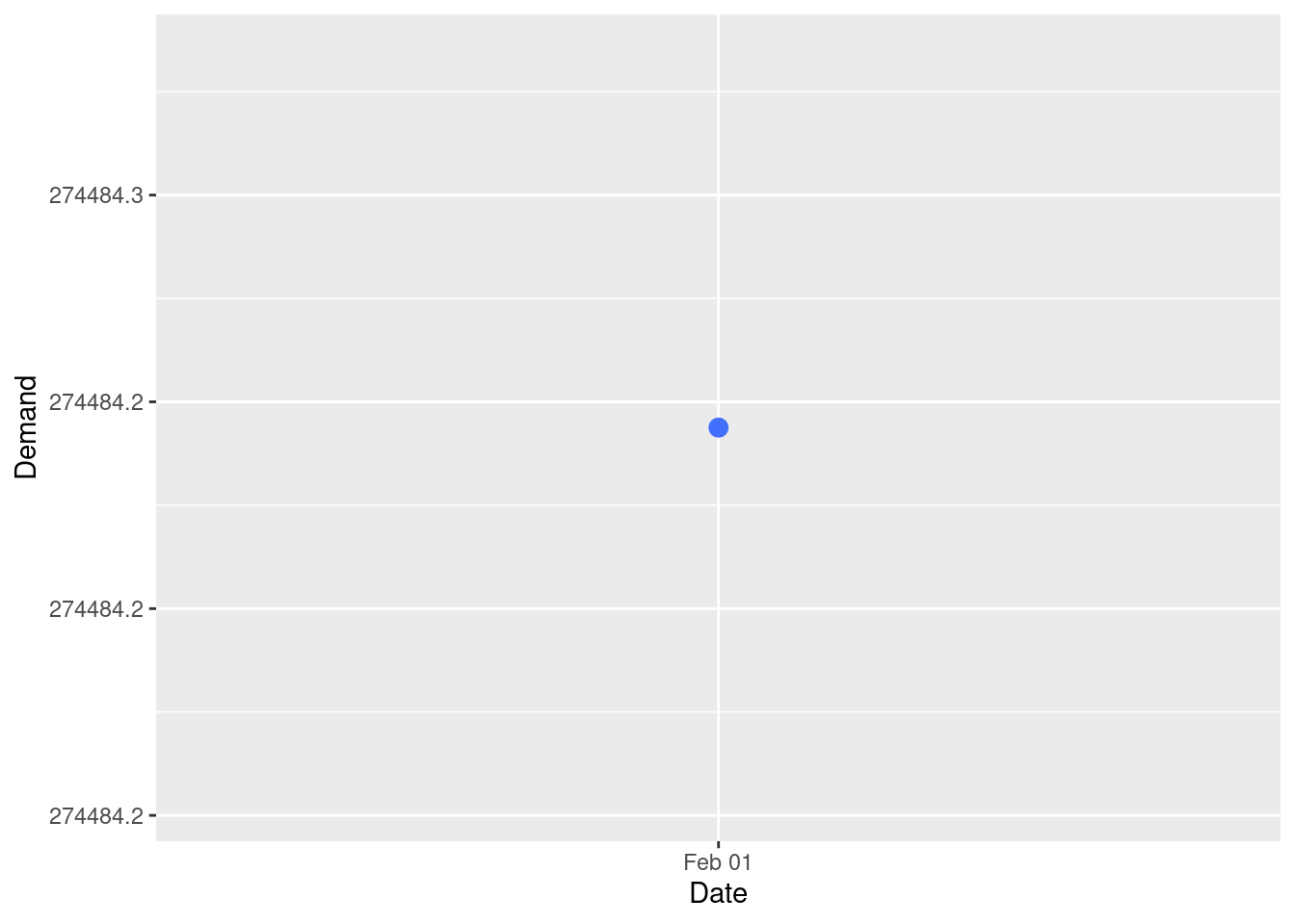
# forecast next day with maximum temperature = 35 degrees Celsius
jan14_vic_elec %>%
     model(tslm = TSLM(Demand ~ Temperature)) %>%
     forecast(
          new_data(jan14_vic_elec, 1) %>%
               mutate(Temperature = 35)
     ) %>%
     autoplot()
## Warning: Computation failed in `stat_interval()`.
## Caused by error in `trans$transform()`:
## ! `transform_date()` works with objects of class <Date> only
## Warning in min(x, na.rm = na.rm): no non-missing arguments to min; returning
## Inf
## Warning in max(x, na.rm = na.rm): no non-missing arguments to max; returning
## -Inf
## Warning in min(x, na.rm = na.rm): no non-missing arguments to min; returning
## Inf
## Warning in max(x, na.rm = na.rm): no non-missing arguments to max; returning
## -Inf
## Warning in min(x, na.rm = na.rm): no non-missing arguments to min; returning
## Inf
## Warning in max(x, na.rm = na.rm): no non-missing arguments to max; returning
## -Inf
- Give prediction intervals for your forecasts.
vic_elec %>%
     filter(yearmonth(Time) == yearmonth("2014 Feb")) %>%
     index_by(Date = as_date(Time)) %>%
     summarise(
          Demand = sum(Demand),
          Temperature = max(Temperature) # select maximum temperature
     ) %>%
     slice(1)
## # A tsibble: 1 x 3 [1D]
##   Date        Demand Temperature
##   <date>       <dbl>       <dbl>
## 1 2014-02-01 241283.        29.2
# forecast demand for maximum temperature = 15 degrees Celsius --> 151,398 (mean)
# forecast demand for maximum temperature = 35 degrees Celsius --> 274,484 (mean)
# actual demand for Feb 1, 2014 --> 241,283 with maximum temperature of 29.2 degrees Celsius
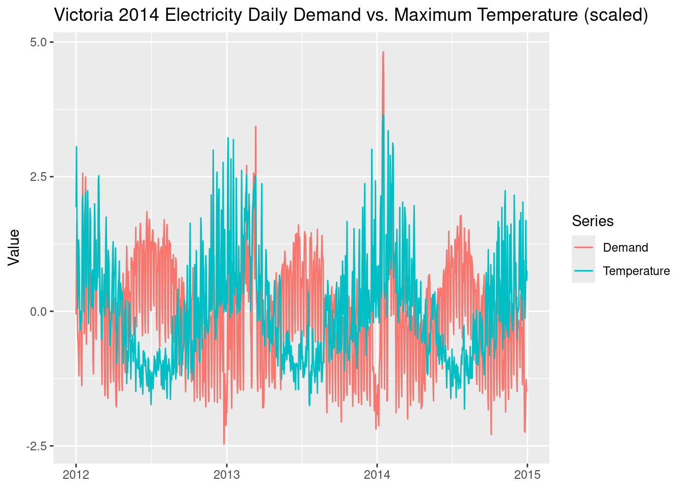
- Plot Demand vs Temperature for all of the available data in vic_elec aggregated to daily total demand and maximum temperature. What does this say about your model?
vic_elec %>%
     select(Date, Demand, Temperature) %>%
     index_by(Date) %>%
     summarise(
          Demand = sum(Demand),
          Temperature = max(Temperature) # select maximum temperature
     ) %>%
     mutate(
          Demand = scale(Demand),
          Temperature = scale(Temperature)
     ) %>%
     pivot_longer(c(Demand, Temperature), names_to = 'Series') %>%
     autoplot(value) +
     labs(x = NULL,
          y = 'Value',
          title = 'Victoria 2014 Electricity Daily Demand vs. Maximum Temperature (scaled)')
fit_trends <- jan14_vic_elec |>
  model(
    linear = TSLM(Demand ~ trend()),
    exponential = TSLM(log(Demand) ~ trend()),
    piecewise = TSLM(Demand ~ trend(knots = c(1950, 1980)))
  )
fc_trends <- fit_trends |> forecast(h = 10)
## Warning: There was 1 warning in `mutate()`.
## ℹ In argument: `piecewise = (function (object, ...) ...`.
## Caused by warning:
## ! prediction from a rank-deficient fit may be misleading