7.3 Multiple Linear Regression Model

Model: \(y_t=\beta_0+\beta_1x_{1,t}+\beta_2x_{2,t}+...+\beta_kx_{k,t}+\epsilon_t\)

\(\beta_0\) is the intercept \(\beta_k\) are the slopes

us_change |>
  pivot_longer(c(-Consumption,-Quarter)) |> # count(name)
  ggplot(aes(value, Consumption, colour = name)) +
  geom_point(shape=21,stroke=0.5,fill="white") +
  geom_smooth(method = "lm",linewidth=0.5,fill="grey80")+
  facet_wrap(~name, scales = "free") +
  theme(legend.position = "none")

## `geom_smooth()` using formula = 'y ~ x'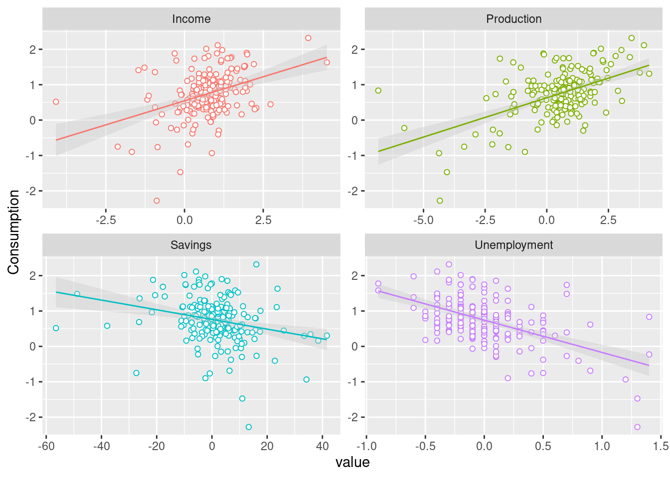

fit_m <- lm(Consumption ~ Income+Production+Savings+Unemployment,data=us_change)

fit_m%>%summary()

## 
## Call:
## lm(formula = Consumption ~ Income + Production + Savings + Unemployment, 
##     data = us_change)
## 
## Residuals:
##      Min       1Q   Median       3Q      Max 
## -0.90555 -0.15821 -0.03608  0.13618  1.15471 
## 
## Coefficients:
##               Estimate Std. Error t value Pr(>|t|)    
## (Intercept)   0.253105   0.034470   7.343 5.71e-12 ***
## Income        0.740583   0.040115  18.461  < 2e-16 ***
## Production    0.047173   0.023142   2.038   0.0429 *  
## Savings      -0.052890   0.002924 -18.088  < 2e-16 ***
## Unemployment -0.174685   0.095511  -1.829   0.0689 .  
## ---
## Signif. codes:  0 '***' 0.001 '**' 0.01 '*' 0.05 '.' 0.1 ' ' 1
## 
## Residual standard error: 0.3102 on 193 degrees of freedom
## Multiple R-squared:  0.7683, Adjusted R-squared:  0.7635 
## F-statistic:   160 on 4 and 193 DF,  p-value: < 2.2e-16