7.2 US consumption expenditure

Time series of quarterly percentage changes (growth rates) of real personal consumption expenditure

us_change |>
  pivot_longer(c(Consumption, Income), names_to="Series") |>
  autoplot(value) +
  labs(y = "% change")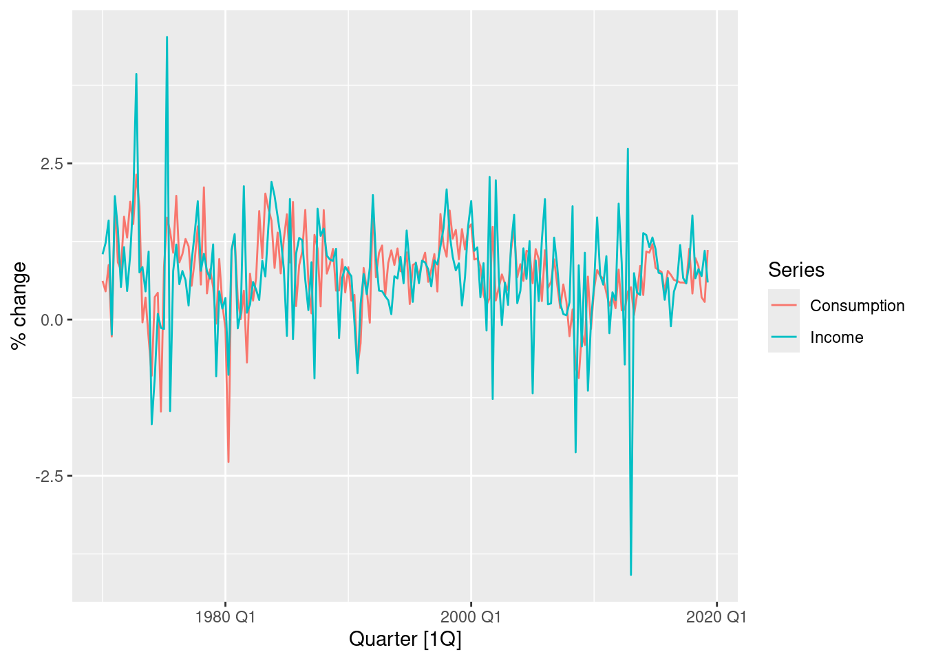

mean(us_change$Consumption)

## [1] 0.7424821

fit <- lm(Consumption~Income, data=us_change)
fit

## 
## Call:
## lm(formula = Consumption ~ Income, data = us_change)
## 
## Coefficients:
## (Intercept)       Income  
##      0.5445       0.2718

us_change |>
  ggplot(aes(x = Income, y = Consumption)) +
  labs(y = "Consumption (quarterly % change)",
       x = "Income (quarterly % change)") +
  geom_point() +
  geom_smooth(method = "lm", se = FALSE)

## `geom_smooth()` using formula = 'y ~ x'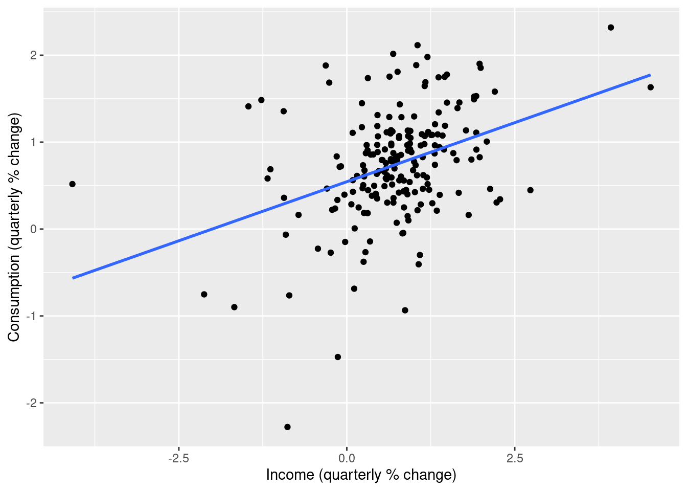

us_change |>
  model(TSLM(Consumption ~ Income)) |>
  report()

## Series: Consumption 
## Model: TSLM 
## 
## Residuals:
##      Min       1Q   Median       3Q      Max 
## -2.58236 -0.27777  0.01862  0.32330  1.42229 
## 
## Coefficients:
##             Estimate Std. Error t value Pr(>|t|)    
## (Intercept)  0.54454    0.05403  10.079  < 2e-16 ***
## Income       0.27183    0.04673   5.817  2.4e-08 ***
## ---
## Signif. codes:  0 '***' 0.001 '**' 0.01 '*' 0.05 '.' 0.1 ' ' 1
## 
## Residual standard error: 0.5905 on 196 degrees of freedom
## Multiple R-squared: 0.1472,  Adjusted R-squared: 0.1429
## F-statistic: 33.84 on 1 and 196 DF, p-value: 2.4022e-08