3.5 Exercises
3.5.1 Exercise 5
For the following series, find an appropriate Box-Cox transformation in order to stabilise the variance.
The Box-Cox transformation uses a separate estimation procedure prior to the logistic regression model that can put the predictors on a new scale. (http://www.feat.engineering/a-simple-example.html) The estimation procedure recommended that both predictors should be used on the inverse scale (i.e., 1/A instead of A).
Data to use:
- Tobacco from aus_production
- Economy class passengers between Melbourne and Sydney from ansett
- Pedestrian counts at Southern Cross Station from pedestrian.
3.5.1.1 Tobacco from aus_production
To find an appropriate Box-Cox transformation we use the Guerrero method to set the \(\lambda\) value.
?features
features(Tobacco, features = guerrero) %>%
               pull(lambda_guerrero)
lambda_tobacco <- aus_production %>%
                   features(Tobacco, features = guerrero) %>%
                   pull(lambda_guerrero)
lambda_tobacco
## [1] 0.9264636## [1] 3003.912 2978.861 3042.256 3246.124 3191.013 3230.234Tobacco %>%
autoplot(box_cox(Tobacco, lambda_tobacco)) +
labs(title=paste("Lambda with feature function method Guerrero =",
round(lambda_tobacco,4)),
x="Time(Quarters)",y="Tobacco values - box_cox transf")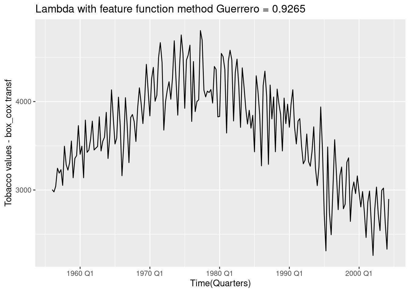
with forecast package:
BoxCox.lambda()with Guerrero method set: \(\lambda\) = 0.7099289
library(forecast)
# Tobacco
fc_lambda <- BoxCox.lambda(Tobacco$Tobacco,method = "guerrero",
                                                      lower=0)
fc_lambda
## [1] 0.7099431Tobacco %>%
autoplot(box_cox(Tobacco, lambda = fc_lambda)) +
labs(title=paste("Lambda with forecast method Guerrero =",
round(fc_lambda,4)),
x="Time(Quarters)",y="Tobacco values - box_cox transf")
with TidyModels
library(tidymodels)
recipe(Tobacco~.,Tobacco)%>%
step_BoxCox(Tobacco,lambdas = fc_lambda)%>%
prep()%>%
juice() %>%
as_tsibble() %>%
autoplot(Tobacco)+
labs(title="Box-Cox transformed")
p <- Tobacco %>%
autoplot(Tobacco)+
labs(title="Original data")
p1 <- Tobacco %>%
autoplot(box_cox(Tobacco, lambda = fc_lambda)) +
labs(title=paste("Lambda with forecast method Guerrero =",
round(fc_lambda,4)),
x="Time(Quarters)",y="Tobacco values - box_cox transf")
library(patchwork)
p|p1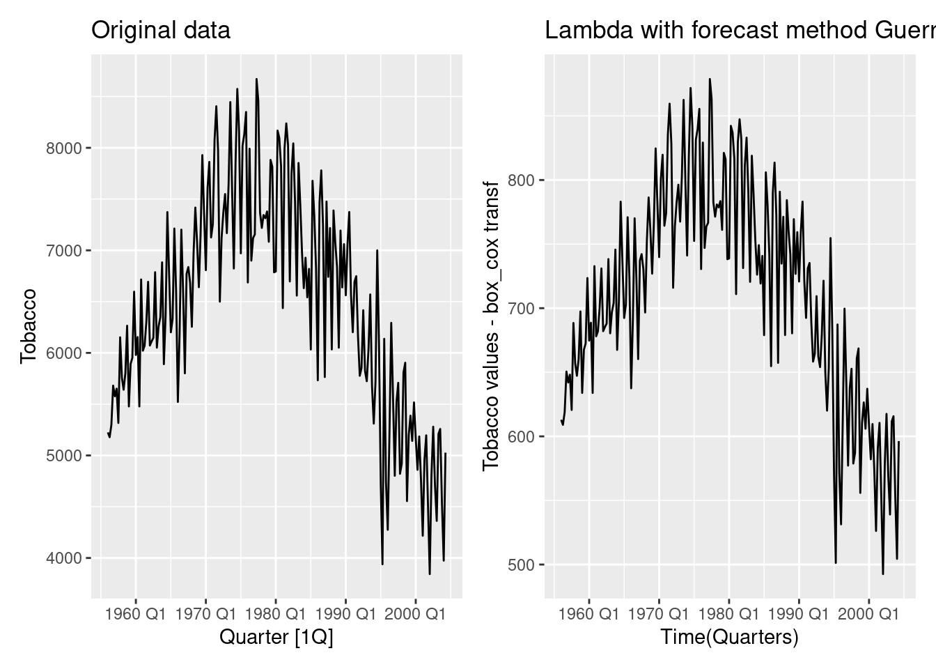
3.5.1.2 Economy class passengers between Melbourne and Sydney from ansett
lambda_class <- ansett %>%
                 filter(Class == "Economy",
                        Airports == "MEL-SYD")%>%
                 features(Passengers, features = guerrero) %>%
                 pull(lambda_guerrero)
ansett %>%
  filter(Class == "Economy",
         Airports == "MEL-SYD")%>%
  mutate(Passengers = Passengers/1000) %>%
autoplot(box_cox(Passengers, lambda = lambda_class)) 
3.5.1.3 Pedestrian counts at Southern Cross Station from pedestrian
lambda_count <- pedestrian %>%
                filter(Sensor == "Southern Cross Station") %>%
                 features(Count, features = guerrero) %>%
                 pull(lambda_guerrero)
pedestrian %>%
  filter(Sensor == "Southern Cross Station") %>%
  autoplot(box_cox(Count,lambda_count))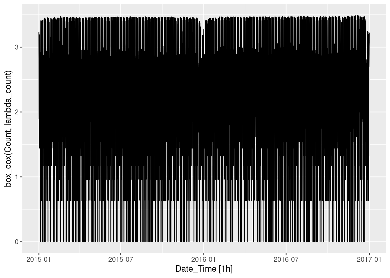
3.5.2 Exrecise 10
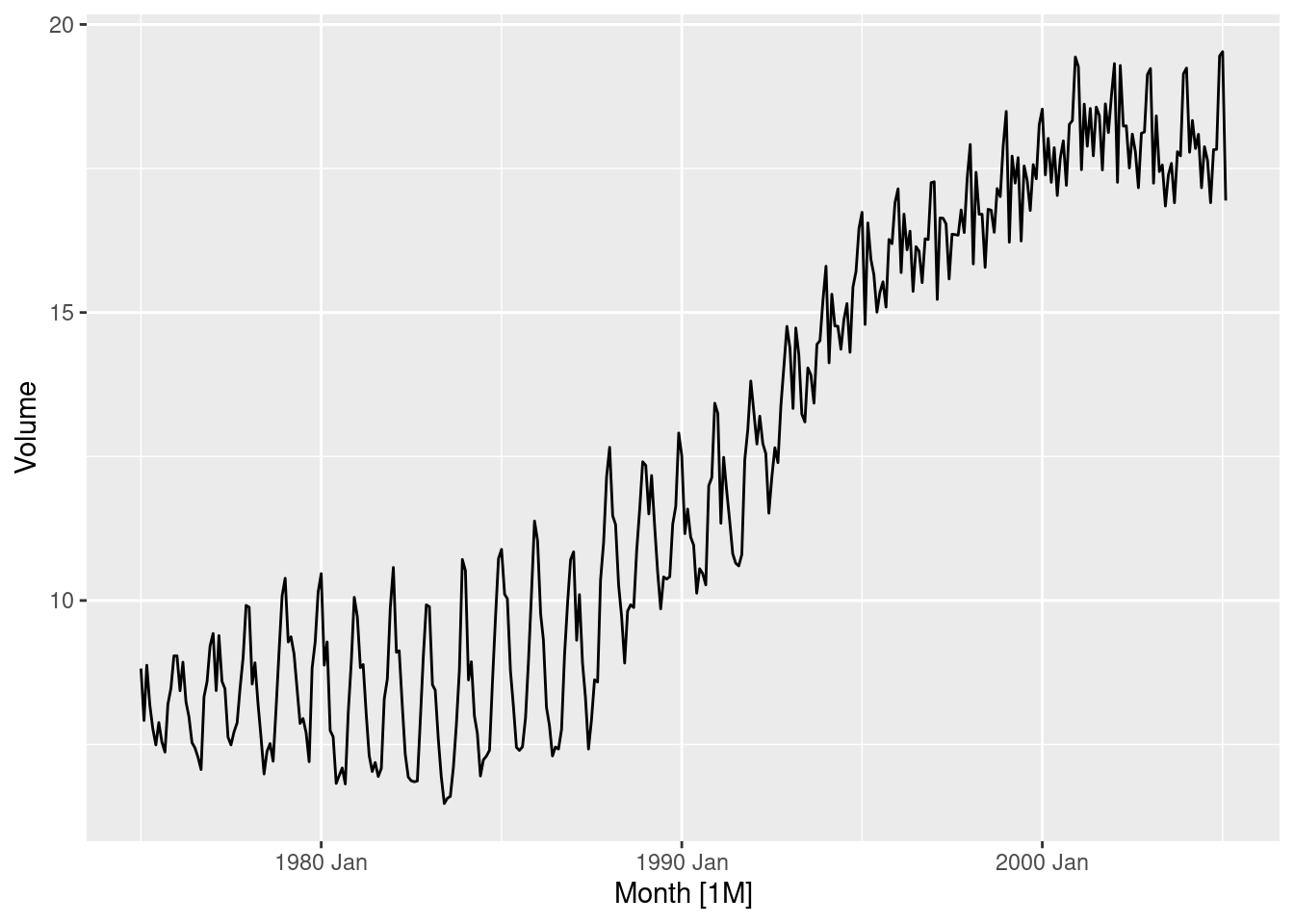
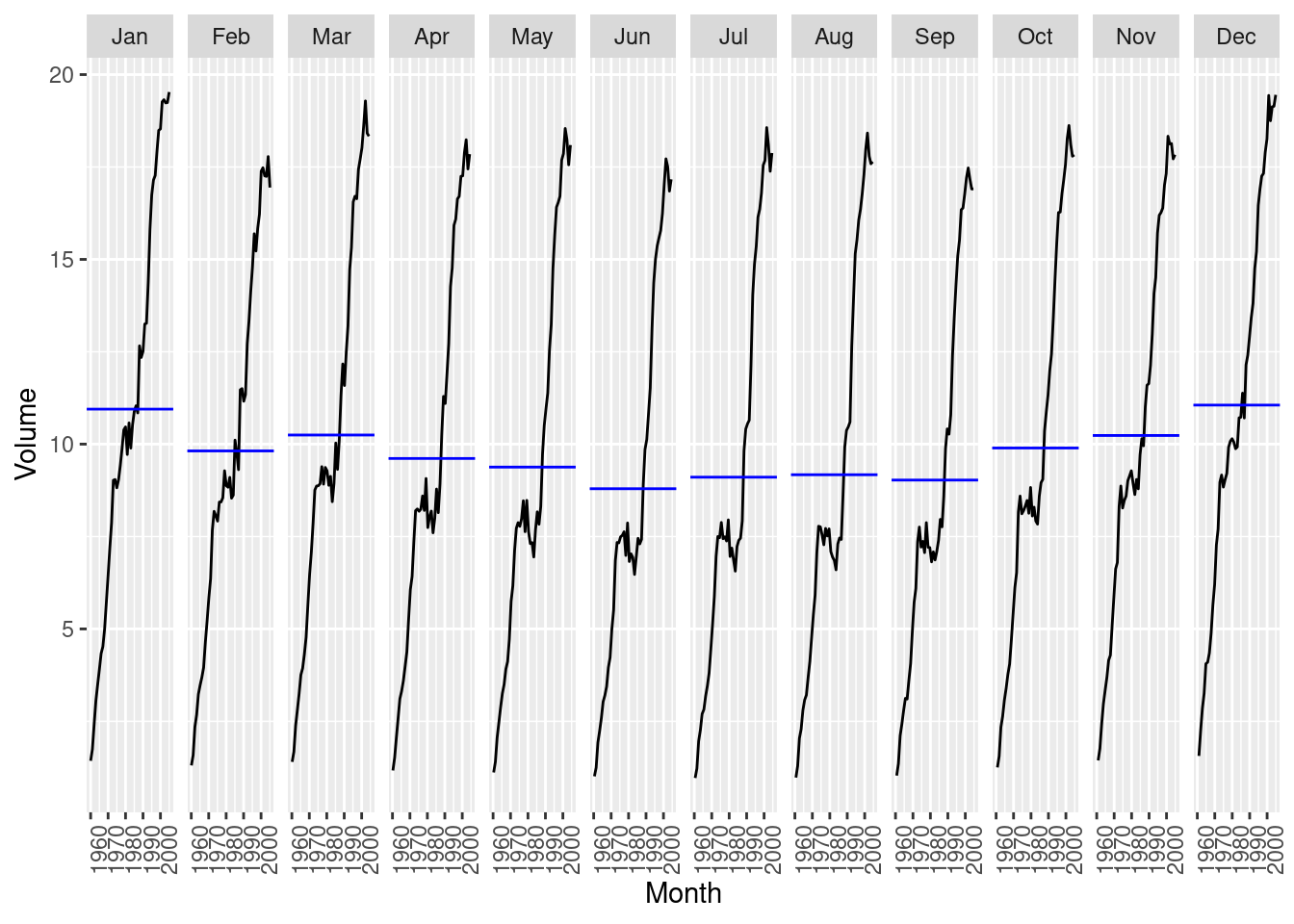
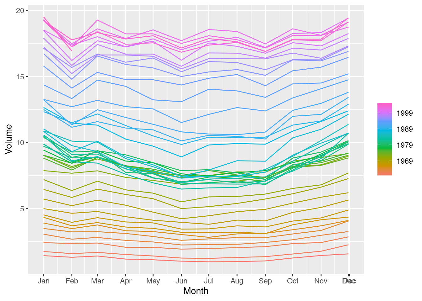
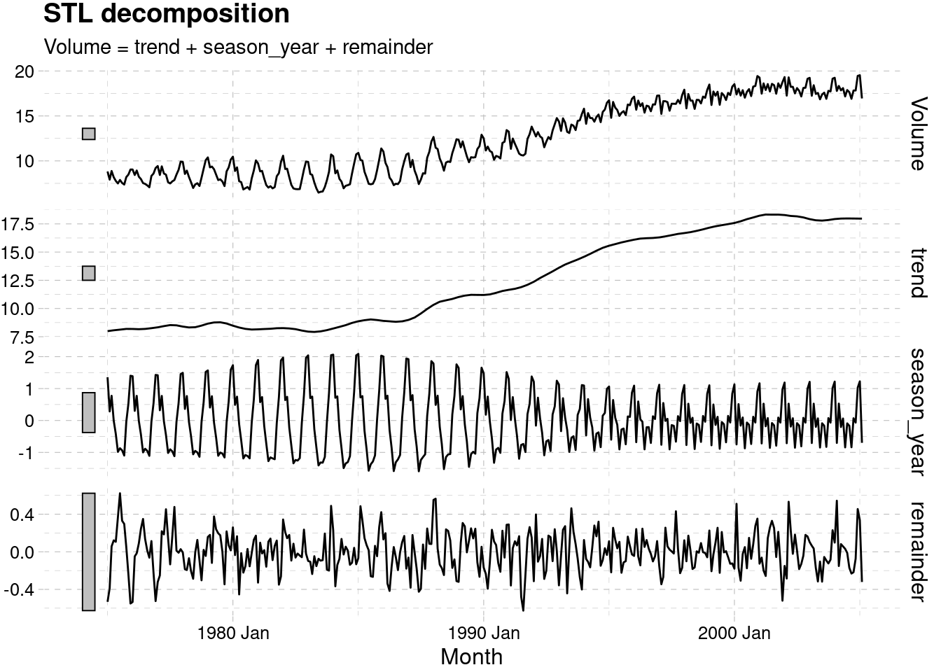
This exercise uses the canadian_gas data (monthly Canadian gas production in billions of cubic metres, January 1960 – February 2005).
Plot the data using autoplot(), gg_subseries() and gg_season() to look at the effect of the changing seasonality over time.
Do an STL decomposition of the data. You will need to choose a seasonal window to allow for the changing shape of the seasonal component.
- How does the seasonal shape change over time? [Hint: Try plotting the seasonal component using gg_season().]
- Can you produce a plausible seasonally adjusted series?
- Compare the results with those obtained using SEATS and X-11.
- How are they different?
3.5.2.1 STL Decomposition
Window greater than 1975
 Full
Full
dcmp_canadian_gas <- canadian_gas %>%
 model(stl = STL(Volume))
components(dcmp_canadian_gas) %>%
  autoplot()+
  ggthemes::theme_pander()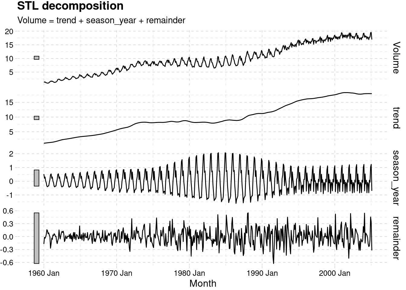
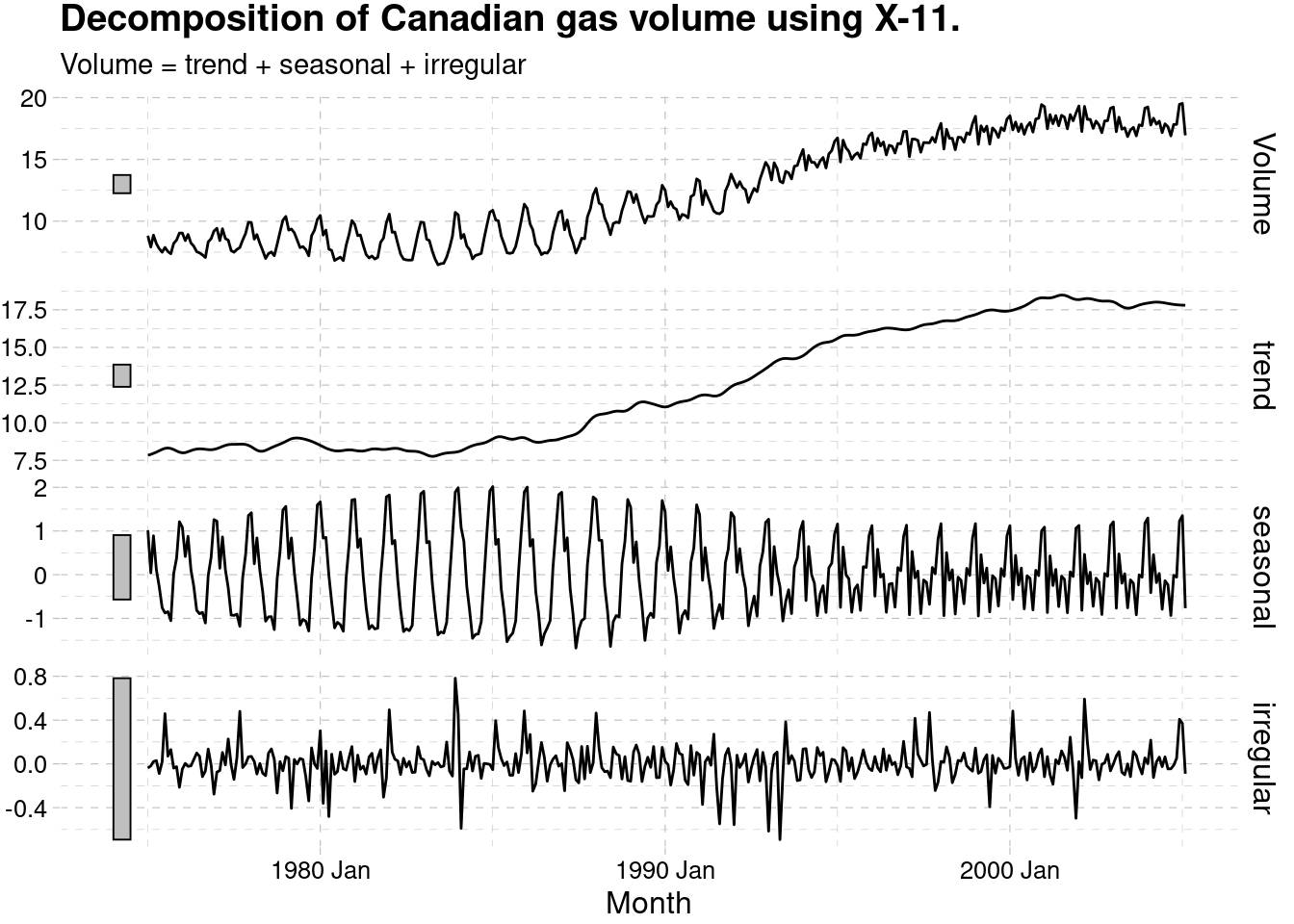
3.5.2.2 X11
x11_dcmp_canadian_gas_w <- canadian_gas %>%
  filter(year(Month) >= 1975) %>%
  model(x11 = X_13ARIMA_SEATS(Volume ~ x11())) %>%
  components()


autoplot(x11_dcmp_canadian_gas_w) +
  labs(title =
    "Decomposition of Canadian gas volume using X-11.")+
  ggthemes::theme_pander()
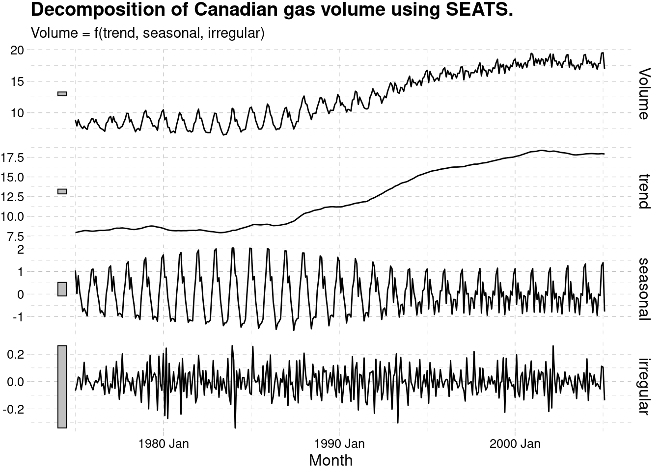
3.5.2.3 SEATS
seats_dcmp_canadian_gas_w <- canadian_gas %>%
  filter(year(Month) >= 1975) %>%
 model(seats = X_13ARIMA_SEATS(Volume ~ seats())) %>%
  components()


autoplot(seats_dcmp_canadian_gas_w) +
  labs(title =
    "Decomposition of Canadian gas volume using SEATS.")+
  ggthemes::theme_pander()
Data to use:
- Tobacco from aus_production
- Economy class passengers between Melbourne and Sydney from ansett
- Pedestrian counts at Southern Cross Station from pedestrian.
3.5.2.4 Tobacco from aus_production
To find an appropriate Box-Cox transformation we use the Guerrero method to set the \(\lambda\) value.
?features
features(Tobacco, features = guerrero) %>%
               pull(lambda_guerrero)
lambda_tobacco <- aus_production %>%
                   features(Tobacco, features = guerrero) %>%
                   pull(lambda_guerrero)
lambda_tobacco
## [1] 0.9264636## [1] 3003.912 2978.861 3042.256 3246.124 3191.013 3230.234Tobacco %>%
autoplot(box_cox(Tobacco, lambda_tobacco)) +
labs(title=paste("Lambda with feature function method Guerrero =",
round(lambda_tobacco,4)),
x="Time(Quarters)",y="Tobacco values - box_cox transf")
with forecast package:
BoxCox.lambda()with Guerrero method set: \(\lambda\) = 0.7099289
library(forecast)
# Tobacco
fc_lambda <- BoxCox.lambda(Tobacco$Tobacco,method = "guerrero",
                                                      lower=0)
fc_lambda
## [1] 0.7099431Tobacco %>%
autoplot(box_cox(Tobacco, lambda = fc_lambda)) +
labs(title=paste("Lambda with forecast method Guerrero =",
round(fc_lambda,4)),
x="Time(Quarters)",y="Tobacco values - box_cox transf")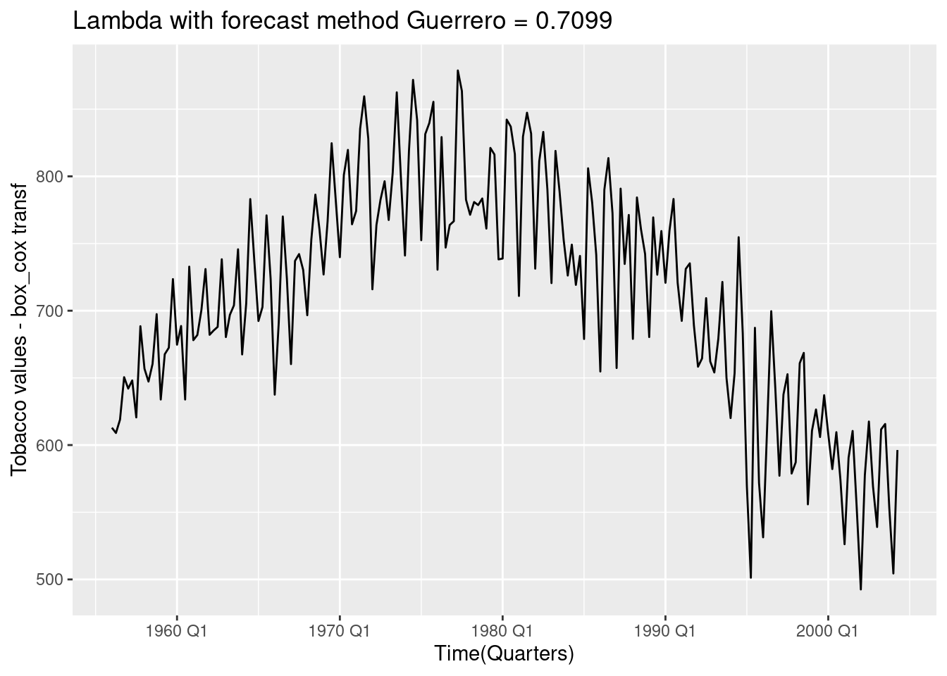
with TidyModels
library(tidymodels)
recipe(Tobacco~.,Tobacco)%>%
step_BoxCox(Tobacco,lambdas = fc_lambda)%>%
prep()%>%
juice() %>%
as_tsibble() %>%
autoplot(Tobacco)+
labs(title="Box-Cox transformed")
p <- Tobacco %>%
autoplot(Tobacco)+
labs(title="Original data")
p1 <- Tobacco %>%
autoplot(box_cox(Tobacco, lambda = fc_lambda)) +
labs(title=paste("Lambda with forecast method Guerrero =",
round(fc_lambda,4)),
x="Time(Quarters)",y="Tobacco values - box_cox transf")
library(patchwork)
p|p1
3.5.2.5 Economy class passengers between Melbourne and Sydney from ansett
lambda_class <- ansett %>%
                 filter(Class == "Economy",
                        Airports == "MEL-SYD")%>%
                 features(Passengers, features = guerrero) %>%
                 pull(lambda_guerrero)
ansett %>%
  filter(Class == "Economy",
         Airports == "MEL-SYD")%>%
  mutate(Passengers = Passengers/1000) %>%
autoplot(box_cox(Passengers, lambda = lambda_class)) 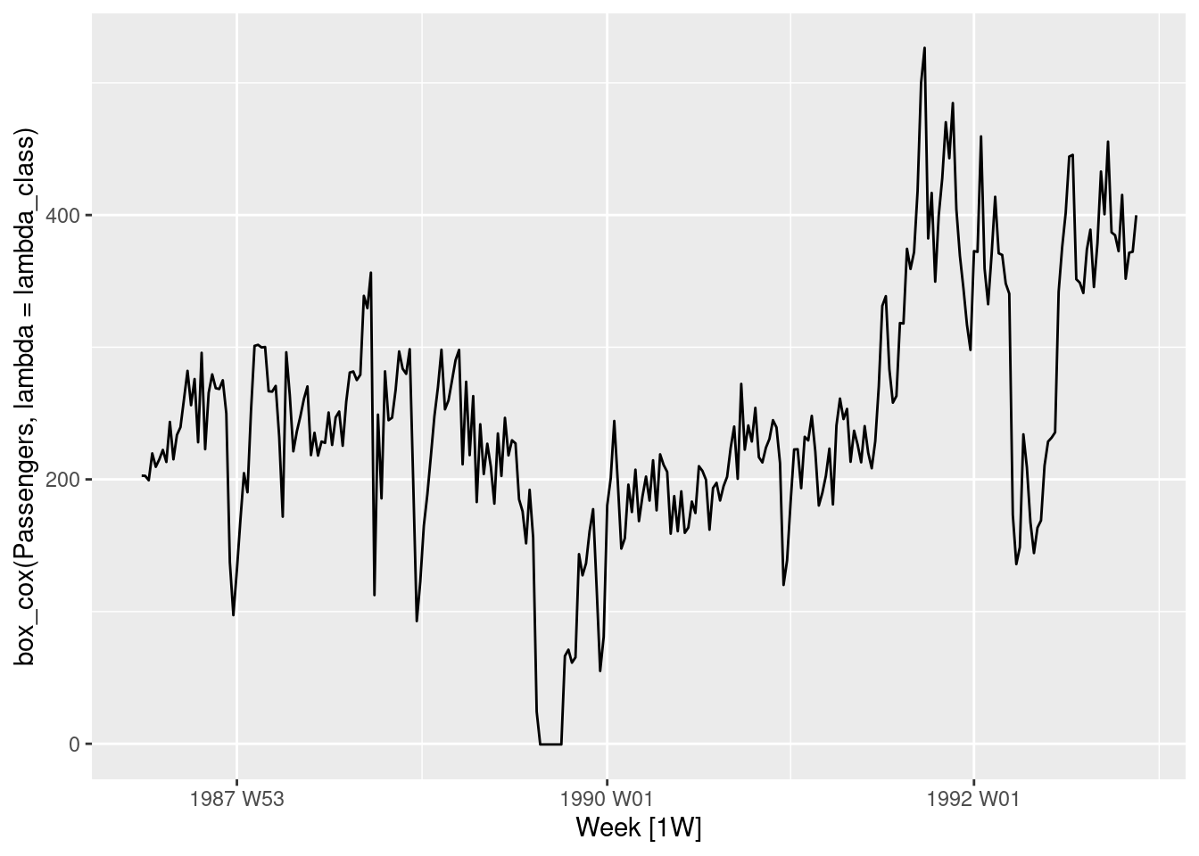
3.5.2.6 Pedestrian counts at Southern Cross Station from pedestrian
lambda_count <- pedestrian %>%
                filter(Sensor == "Southern Cross Station") %>%
                 features(Count, features = guerrero) %>%
                 pull(lambda_guerrero)
pedestrian %>%
  filter(Sensor == "Southern Cross Station") %>%
  autoplot(box_cox(Count,lambda_count))
3.5.3 Exrecise 10
This exercise uses the canadian_gas data (monthly Canadian gas production in billions of cubic metres, January 1960 – February 2005).
Plot the data using autoplot(), gg_subseries() and gg_season() to look at the effect of the changing seasonality over time.
Do an STL decomposition of the data. You will need to choose a seasonal window to allow for the changing shape of the seasonal component.
- How does the seasonal shape change over time? [Hint: Try plotting the seasonal component using gg_season().]
- Can you produce a plausible seasonally adjusted series?
- Compare the results with those obtained using SEATS and X-11.
- How are they different?


3.5.3.1 STL Decomposition
Window greater than 1975
Full
dcmp_canadian_gas <- canadian_gas %>%
 model(stl = STL(Volume))
components(dcmp_canadian_gas) %>%
  autoplot()+
  ggthemes::theme_pander()