4.3 STL features
A time series decomposition can be used to measure the strength of trend and seasonality in a time series. Recall that the decomposition is written as:
\(y_{t} = T_{t} + S_{t} + R_{t}\),
where \(T_{t}\) is the smoothed trend component, \(S_{t}\) is the seasonal component and \(R_{t}\) is a remainder component.
These measures can be useful, for example, when you have a large collection of time series, and you need to find the series with the most trend or the most seasonality.
These and other STL-based features are computed using the
feat_stl()function.
## # A tibble: 304 × 12
## Region State Purpose trend_strength seasonal_strength_year seasonal_peak_year
## <chr> <chr> <chr> <dbl> <dbl> <dbl>
## 1 Adela… Sout… Busine… 0.464 0.407 3
## 2 Adela… Sout… Holiday 0.554 0.619 1
## 3 Adela… Sout… Other 0.746 0.202 2
## 4 Adela… Sout… Visiti… 0.435 0.452 1
## 5 Adela… Sout… Busine… 0.464 0.179 3
## 6 Adela… Sout… Holiday 0.528 0.296 2
## 7 Adela… Sout… Other 0.593 0.404 2
## 8 Adela… Sout… Visiti… 0.488 0.254 0
## 9 Alice… Nort… Busine… 0.534 0.251 0
## 10 Alice… Nort… Holiday 0.381 0.832 3
## # ℹ 294 more rows
## # ℹ 6 more variables: seasonal_trough_year <dbl>, spikiness <dbl>,
## # linearity <dbl>, curvature <dbl>, stl_e_acf1 <dbl>, stl_e_acf10 <dbl>We can then use these features in plots to identify what type of series are heavily trended and what are most seasonal.
tourism %>%
features(Trips, feat_stl) %>%
ggplot(aes(x = trend_strength, y = seasonal_strength_year,
col = Purpose)) +
geom_point() +
facet_wrap(vars(State))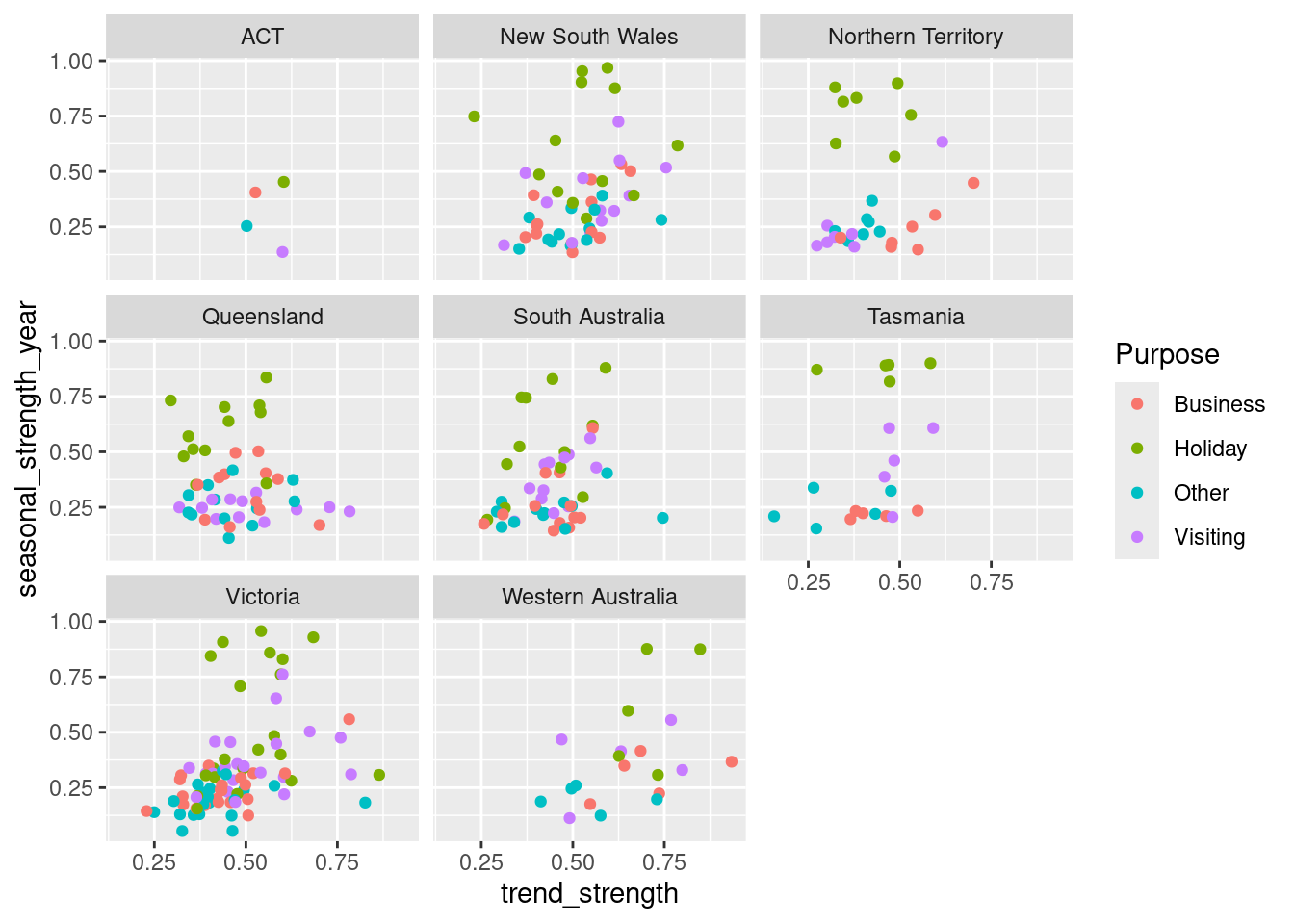
Clearly, holiday series are most seasonal, which is not surprising.
The strongest trends tend to be in Western Australia and Victoria.
The most seasonal series can also be easily identified and plotted.
tourism %>%
     features(Trips, feat_stl) %>%
     filter(
          seasonal_strength_year == max(seasonal_strength_year)
     ) %>%
     left_join(tourism, by = c("State", "Region", "Purpose")) %>%
     ggplot(aes(x = Quarter, y = Trips)) +
     geom_line() +
     facet_grid(vars(State, Region, Purpose))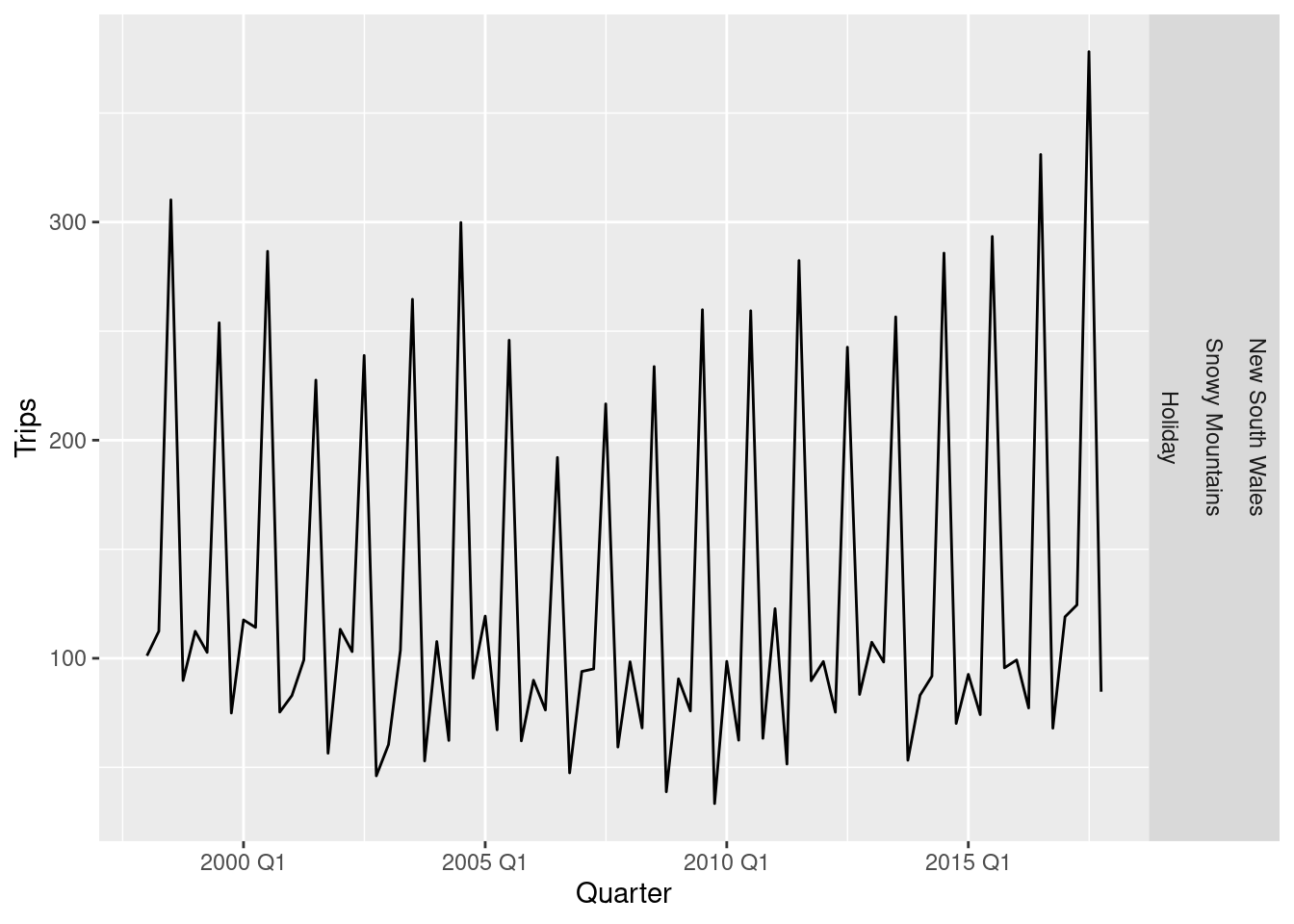
The above plot shows holiday trips to the most popular ski region of Australia.
The feat_stl() function returns several more features other than those discussed above.
- `seasonal_peak_year` indicates the timing of the peaks — which month or quarter contains the largest seasonal component. This tells us something about the nature of the seasonality. In the Australian tourism data, if Quarter 3 is the peak seasonal period, then people are travelling to the region in winter, whereas a peak in Quarter 1 suggests that the region is more popular in summer.

- `seasonal_trough_year` indicates the timing of the troughs — which month or quarter contains the smallest seasonal component.

- `spikiness` measures the prevalence of spikes in the remainder component Rt of the STL decomposition. It is the variance of the leave-one-out variances of Rt.

- `linearity` measures the linearity of the trend component of the STL decomposition. It is based on the coefficient of a linear regression applied to the trend component.

- `curvature` measures the curvature of the trend component of the STL decomposition. It is based on the coefficient from an orthogonal quadratic regression applied to the trend component.

- `stl_e_acf1` is the first autocorrelation coefficient of the remainder series.

- `stl_e_acf10` is the sum of squares of the first ten autocorrelation coefficients of the remainder series.