10.8 Forecast with different levels of TVadverts

Set new data to 20 year-month period time-frame:

new_data(insurance, 20)

Sample TVadverts ranging from 7 to 10:

set.seed(1234)
sample <- sample(7:10,20,replace=T)

Create a newdata with sampled TVadverts:

insurance_future2 <- new_data(insurance, 20) |>
  mutate(TVadverts = sample)
insurance_future2%>%head

## # A tsibble: 6 x 2 [1M]
##      Month TVadverts
##      <mth>     <int>
## 1 2005 May        10
## 2 2005 Jun        10
## 3 2005 Jul         8
## 4 2005 Aug         8
## 5 2005 Sep         7
## 6 2005 Oct        10

Fit the model on sampled TVadverts and plot it:

fit_best <- insurance |>
  model(ARIMA(Quotes ~ pdq(d = 0) +
              TVadverts + lag(TVadverts)))
report(fit_best)

## Series: Quotes 
## Model: LM w/ ARIMA(1,0,2) errors 
## 
## Coefficients:
##          ar1     ma1     ma2  TVadverts  lag(TVadverts)  intercept
##       0.5123  0.9169  0.4591     1.2527          0.1464     2.1554
## s.e.  0.1849  0.2051  0.1895     0.0588          0.0531     0.8595
## 
## sigma^2 estimated as 0.2166:  log likelihood=-23.94
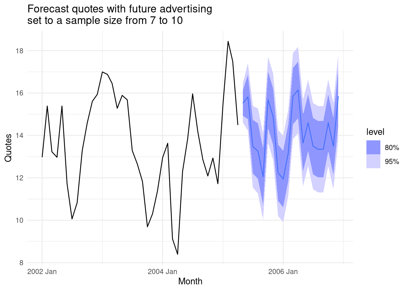
## AIC=61.88   AICc=65.38   BIC=73.7

fit_best |>
  forecast(insurance_future2) |>
  autoplot(insurance) +
  labs(
    y = "Quotes",
    title = "Forecast quotes with future advertising\nset to a sample size from 7 to 10"
  )

Now create a new data with 4 models each with 7,8,9,10 TVadverts:

insurance_future_7 <- new_data(insurance, 20) |>
  mutate(TVadverts = 7)
insurance_future_8 <- new_data(insurance, 20) |>
  mutate(TVadverts = 8)
insurance_future_9 <- new_data(insurance, 20) |>
  mutate(TVadverts = 9)
insurance_future_10 <- new_data(insurance, 20) |>
  mutate(TVadverts = 10)

fit_df_7 <- fit_best |>
  forecast(insurance_future_7)
fit_df_8 <- fit_best |>
  forecast(insurance_future_8)
fit_df_9 <- fit_best |>
  forecast(insurance_future_9)
fit_df_10 <- fit_best |>
  forecast(insurance_future_10)


fit_df_8 <- fit_df_8[2:5]%>%
  rename(TVadverts_8=TVadverts,
         Quotes_8=Quotes,
         .mean_8=.mean)
fit_df_9<- fit_df_9[2:5]%>%
  rename(TVadverts_9=TVadverts,
         Quotes_9=Quotes,
         .mean_9=.mean)
fit_df_10<- fit_df_10[2:5]%>%
  rename(TVadverts_10=TVadverts,
         Quotes_10=Quotes,
         .mean_10=.mean)

insurance_future <- new_data(insurance, 20) |>
  mutate(TVadverts = 8)

fit_best_df<-  fit_best |>
  forecast(insurance_future) %>%
  hilo()

fit_best_df2 <- fit_best_df[2:7]%>%
  mutate(conf_down=as.numeric(sub(".*?(\\d+\\.\\d+).*", "\\1", `80%`)),
         conf_up=as.numeric(sub(".*\\b(\\d+\\.\\d+).*", "\\1", `80%`)),
         conf_down2=as.numeric(sub(".*?(\\d+\\.\\d+).*", "\\1", `95%`)),
         conf_up2=as.numeric(sub(".*\\b(\\d+\\.\\d+).*", "\\1", `95%`)))%>%
  select(-`80%`,-`95%`)

fit_best_df2_int <- fit_best_df2 %>%
  full_join(insurance%>%select(Month,Quotes),by="Month") 

Create new data on those models,

df <- fit_df_7[2:5] %>%
  left_join(fit_df_8, by = "Month") %>%
  left_join(fit_df_9, by = "Month") %>%
  left_join(fit_df_10, by = "Month") %>%
  
  pivot_longer(
    cols = contains("TVadverts"),
    names_to = "TVadverts_num",
    values_to = "TVadverts"
  ) %>%
  pivot_longer(cols = contains(".mean"),
               names_to = "mean_num",
               values_to = ".mean") %>%
  pivot_longer(cols = contains("Quotes"),
               names_to = "Quotes_num",
               values_to = "Quotes") %>%
  distinct() %>%
  arrange(Month)

df %>% head

## # A tibble: 6 × 7
##      Month TVadverts_num TVadverts mean_num .mean Quotes_num      Quotes
##      <mth> <chr>             <dbl> <chr>    <dbl> <chr>           <dist>
## 1 2005 May TVadverts             7 .mean     11.8 Quotes     N(12, 0.22)
## 2 2005 May TVadverts             7 .mean     11.8 Quotes_8   N(13, 0.22)
## 3 2005 May TVadverts             7 .mean     11.8 Quotes_9   N(14, 0.22)
## 4 2005 May TVadverts             7 .mean     11.8 Quotes_10  N(16, 0.22)
## 5 2005 May TVadverts             7 .mean_8   13.0 Quotes     N(12, 0.22)
## 6 2005 May TVadverts             7 .mean_8   13.0 Quotes_8   N(13, 0.22)

And plot it:

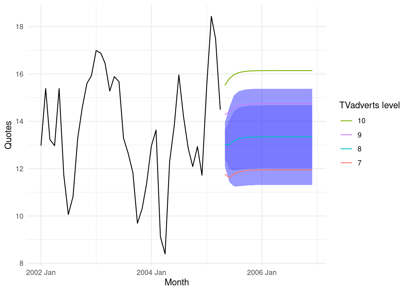
ggplot() +
  geom_ribbon(
    data = fit_best_df2_int,
    mapping = aes(x = Month, ymin = conf_down2, ymax = conf_up2),
    fill = "blue",
    alpha = 0.4
  ) +
  geom_ribbon(
    data = fit_best_df2_int,
    mapping = aes(x = Month, ymin = conf_down, ymax = conf_up),
    fill = "blue",
    alpha = 0.2
  ) +
  geom_line(data = insurance, mapping = aes(x = Month, y = Quotes)) +
  geom_line(
    data = df,
    mapping = aes(
      x = Month,
      y = .mean,
      group = mean_num,
      color = mean_num
    )
  ) +
  scale_color_discrete(
    breaks = c(".mean_10",
               ".mean_9",
               ".mean_8",
               ".mean"),
    label = c(
      ".mean" = "7",
      ".mean_8" = "8",
      ".mean_9" = "9",
      ".mean_10" = "10"
    ),
    name = "TVadverts level"
  )