12.2 Prophet model

The Prophet model it’s a nonlinear regression model available via the {fable.prophet} package, it works best with time series that have strong seasonality and several seasons of historical data. The model is estimated using a Bayesian approach to allow for automatic selection of the change-points and other model characteristics.

\[y_t=g(t)+s(t)+h(t)+\epsilon_t\]

• \(g(t)\) = piecewise-linear trend (or “growth term”)
• \(s(t)\) = seasonal patterns
• \(h(t)\) = holiday effects
• \(\epsilon_t\) = white noise error term

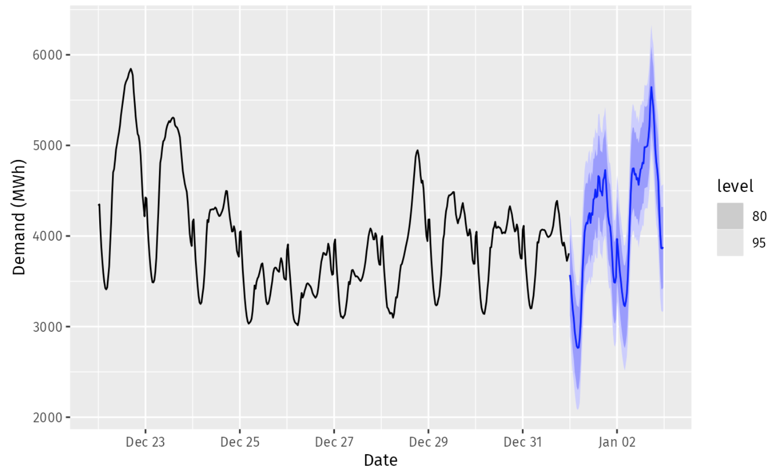
12.2.1 Case Study 3

Quarterly cement production:

library(fable.prophet)

## Loading required package: Rcpp

cement <- aus_production |>
  filter(year(Quarter) >= 1988)
cement%>%head

## # A tsibble: 6 x 7 [1Q]
##   Quarter  Beer Tobacco Bricks Cement Electricity   Gas
##     <qtr> <dbl>   <dbl>  <dbl>  <dbl>       <dbl> <dbl>
## 1 1988 Q1   474    6034    428   1418       33142   116
## 2 1988 Q2   440    7389    519   1625       34664   137
## 3 1988 Q3   447    7077    555   1770       37154   157
## 4 1988 Q4   598    6837    538   1791       35303   125
## 5 1989 Q1   467    6051    510   1621       36905   117
## 6 1989 Q2   439    7193    571   1719       37333   149

train <- cement |>
  filter(year(Quarter) <= 2007)

fit3 <- train |>
  model(
    arima = ARIMA(Cement),
    ets = ETS(Cement),
    prophet = prophet(Cement ~ season(period = 4, 
                                      order = 2,
                                      type = "multiplicative"))
    )

fc3 <- fit3 |> 
  forecast(h = "2 years 6 months")

fc3 |> autoplot(cement)

fc3 |> 
  fabletools::accuracy(cement)

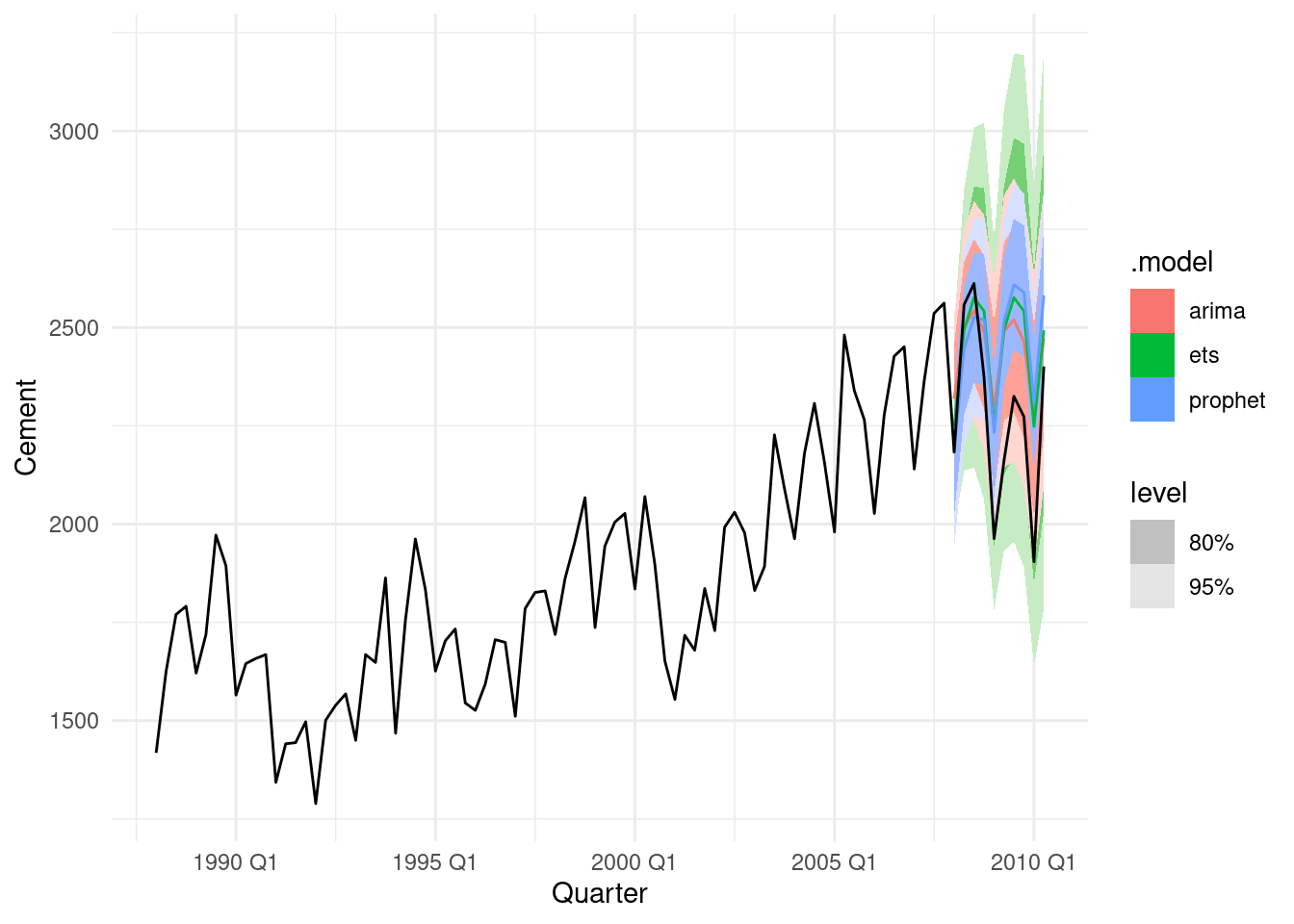
## # A tibble: 3 × 10
##   .model  .type    ME  RMSE   MAE   MPE  MAPE  MASE RMSSE  ACF1
##   <chr>   <chr> <dbl> <dbl> <dbl> <dbl> <dbl> <dbl> <dbl> <dbl>
## 1 arima   Test  -161.  216.  186. -7.71  8.68  1.27  1.26 0.387
## 2 ets     Test  -171.  222.  191. -8.07  8.85  1.30  1.29 0.579
## 3 prophet Test  -176.  248.  215. -8.35  9.89  1.47  1.44 0.702

12.2.2 Case Study 4

Half-hourly electricity demand:

elec <- vic_elec |>
  mutate(
    DOW = wday(Date, label = TRUE),
    Working_Day = !Holiday & !(DOW %in% c("Sat", "Sun")),
    Cooling = pmax(Temperature, 18)
  )

Faster than Dynamic harmonic regression models (DHR).

The Prophet model adds a piecewise linear time trend which is not really appropriate here as we don’t expect the long term forecasts to continue to follow the downward linear trend at the end of the series.

fit4 <- elec |>
  model(
    prophet(Demand ~ Temperature + Cooling + Working_Day +
            season(period = "day", order = 10) +
            season(period = "week", order = 5) +
            season(period = "year", order = 3))
  )

fc <- fit4 |>
  forecast(new_data = elec_newdata)