12.5 Bootstrapping and bagging

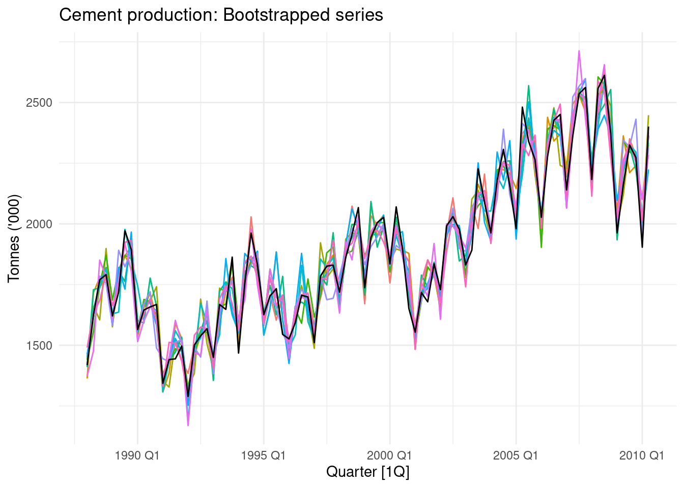
It is a transformation of the time series.

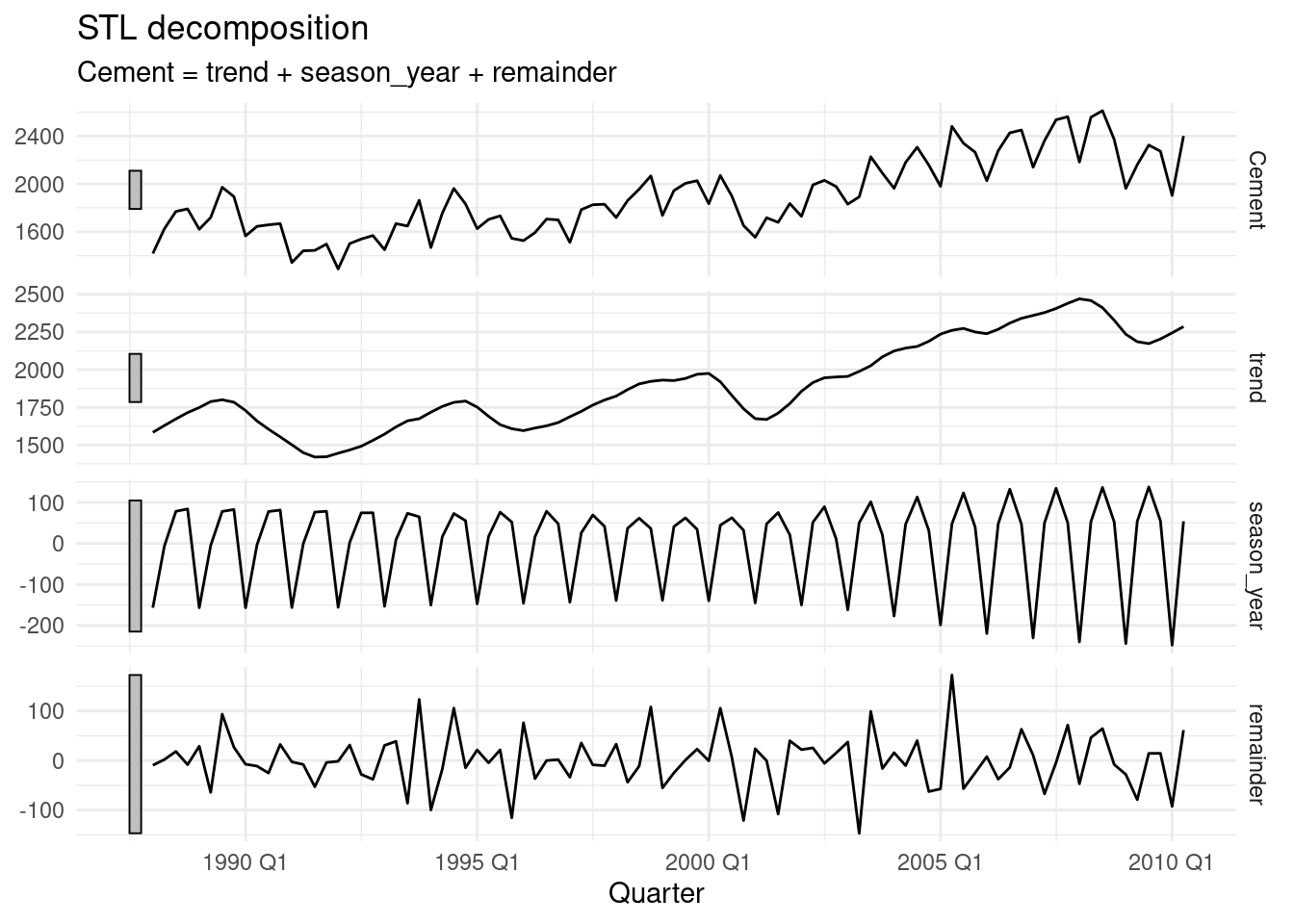
The series is decomposed into trend, seasonal and remainder components using STL.

And then the remainder is bootstrapped to obtain a shuffled versions of it.

12.5.1 Case Study 7

Consider the quarterly cement production in Australia from 1988 Q1 to 2010 Q2. First we check, that the decomposition has adequately captured the trend and seasonality, and that there is no obvious remaining signal in the remainder series.

au_cement <- aus_production%>%
   filter(year(Quarter) >= 1988) |>
  select(Cement)

au_cement%>%head

## # A tsibble: 6 x 2 [1Q]
##   Cement Quarter
##    <dbl>   <qtr>
## 1   1418 1988 Q1
## 2   1625 1988 Q2
## 3   1770 1988 Q3
## 4   1791 1988 Q4
## 5   1621 1989 Q1
## 6   1719 1989 Q2

fit7 <- au_cement %>%
  model(stl=STL(Cement))

Time series decomposition

fit7 %>%
  components() |>
  autoplot()

12.5.1.1 Generate several bootstrapped versions of the data

fit7 |>
  generate(new_data = au_cement, times = 10,
           bootstrap_block_size = 8) |>
  autoplot(.sim) +
  autolayer(au_cement, Cement) +
  guides(colour = "none") +
  labs(title = "Cement production: Bootstrapped series",
       y="Tonnes ('000)")

12.5.2 Bagging = bootstrap aggregating

To improve forecast accuracy, take the forecast of each of the additional time series, and calculate the average the resulting forecasts.

sim <- fit7 %>%
  generate(new_data = au_cement, times = 100,
           bootstrap_block_size = 8) |>
  select(-.model, -Cement)
sim%>%head

## # A tsibble: 6 x 3 [1Q]
## # Key:       .rep [1]
##   .rep  Quarter  .sim
##   <chr>   <qtr> <dbl>
## 1 1     1988 Q1 1466.
## 2 1     1988 Q2 1537.
## 3 1     1988 Q3 1875.
## 4 1     1988 Q4 1700.
## 5 1     1989 Q1 1575.
## 6 1     1989 Q2 1889.

fit an ETS model

ets_forecasts <- sim |>
  model(ets = ETS(.sim)) |>
  forecast(h = 12)

ets_forecasts |>
  update_tsibble(key = .rep) |>
  autoplot(.mean) +
  autolayer(au_cement, Cement) +
  guides(colour = "none") +
  labs(title = "Cement production: bootstrapped forecasts",
       y="Tonnes ('000)")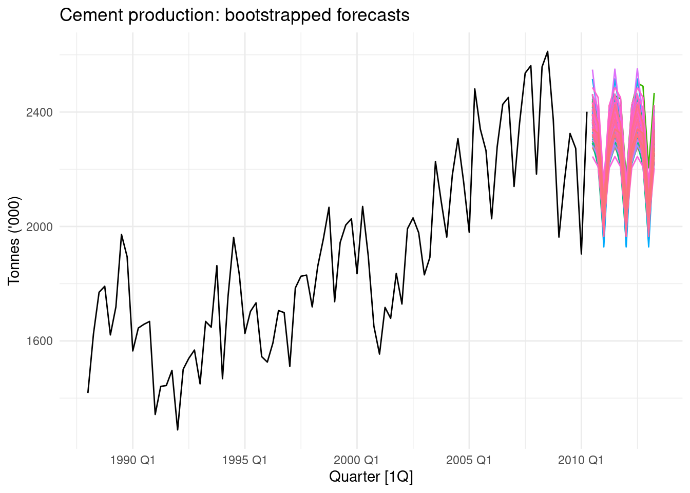

Avg the forecasts

bagged <- ets_forecasts |>
  summarise(bagged_mean = mean(.mean))

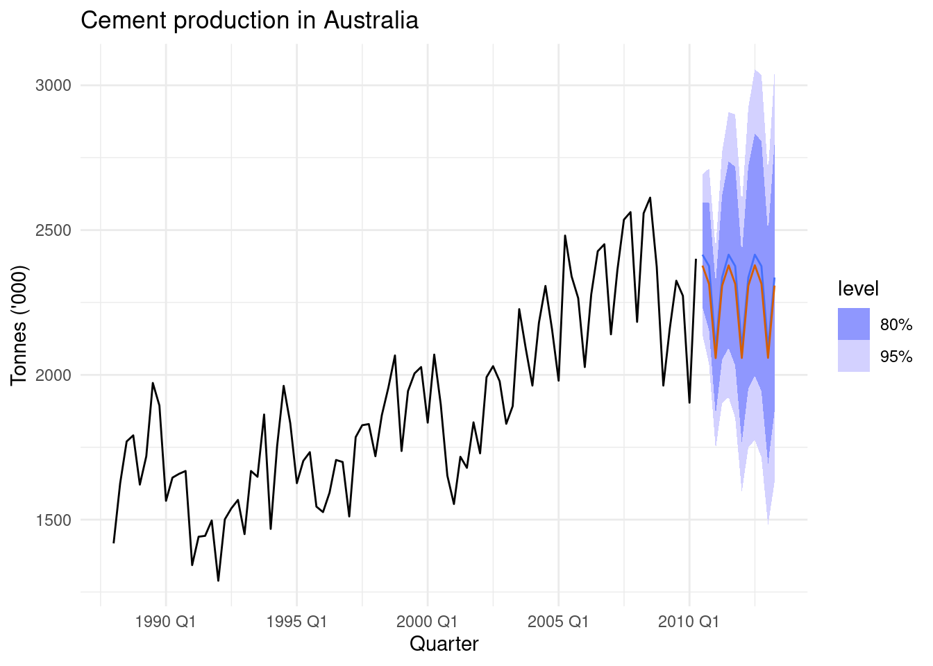
bagging gives better forecasts than just applying ETS() directly.

au_cement |>
  model(ets = ETS(Cement)) |>
  forecast(h = 12) |>
  autoplot(au_cement) +
  autolayer(bagged, bagged_mean, col = "#D55E00") +
  labs(title = "Cement production in Australia",
       y="Tonnes ('000)")