3.2 Time series components
Time series are made of three components:
- a trend-cycle component \(T_t\)
- a seasonal component \(S_t\)
- a remainder component \(R_t\)
3.2.1 Additive decomposition
When the variation around the trend-cycle does not vary with the level of the time series.
\[y_t=S_t+T_t+R_t\]
3.2.2 Multiplicative decomposition
When the variation in the seasonal pattern, or the variation around the trend-cycle, appears to be proportional to the level of the time series.
\[y_t=S_t*T_t*R_t\] An alternative can be a log transformation
\[log(y_t)=log(S_t)+log(T_t)+log(R_t)\]
3.2.3 Example: Employment in the US retail sector
A nice introduction to the use of the {fpp3} package by the author is in the section Example at minute 13.11 here: Dr. Rob J. Hyndman - Ensemble Forecasts with {fable}
Data
## # A tsibble: 6 x 4 [1M]
## # Key:       Series_ID [1]
##      Month Series_ID     Title         Employed
##      <mth> <chr>         <chr>            <dbl>
## 1 1939 Jan CEU0500000001 Total Private    25338
## 2 1939 Feb CEU0500000001 Total Private    25447
## 3 1939 Mar CEU0500000001 Total Private    25833
## 4 1939 Apr CEU0500000001 Total Private    25801
## 5 1939 May CEU0500000001 Total Private    26113
## 6 1939 Jun CEU0500000001 Total Private    26485
3.2.3.1 STL decomposition method
Seasonal and Trend decomposition using Loess.
Some interesting information about the STL model:
- it is additive
- it is iterative and relies on the alternate estimation of the trend
- the seasonal components are locally estimated scatterplot smoothing (Loess)
- it estimates nonlinear relationships
- the seasonal component is allowed to change over time
- it is composed of seasonal patterns estimated based on k consecutive seasonal cycles
- k controls how rapidly the seasonal component can change
- it is robust to outliers and missing data
- it is able to decompose time series with seasonality of any frequency, and provides implementation using numerical methods instead of mathematical modeling.
More info here: R. B. Cleveland et al. (1990)
The command used is:
model(stl = STL(<formula>))us_employment%>% #year(Month) >= 1990,
filter(Title == "Retail Trade") %>%
select(-Series_ID) %>%
autoplot()## Plot variable not specified, automatically selected `.vars = Employed`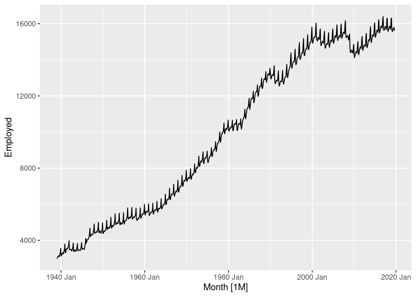
us_retail_employment <- us_employment %>%
  filter(year(Month) >= 1990, Title == "Retail Trade") %>%
  select(-Series_ID)


dcmp <- us_retail_employment %>%
  model(stl = STL(Employed))


components(dcmp) %>%
  autoplot()+
  ggthemes::theme_pander()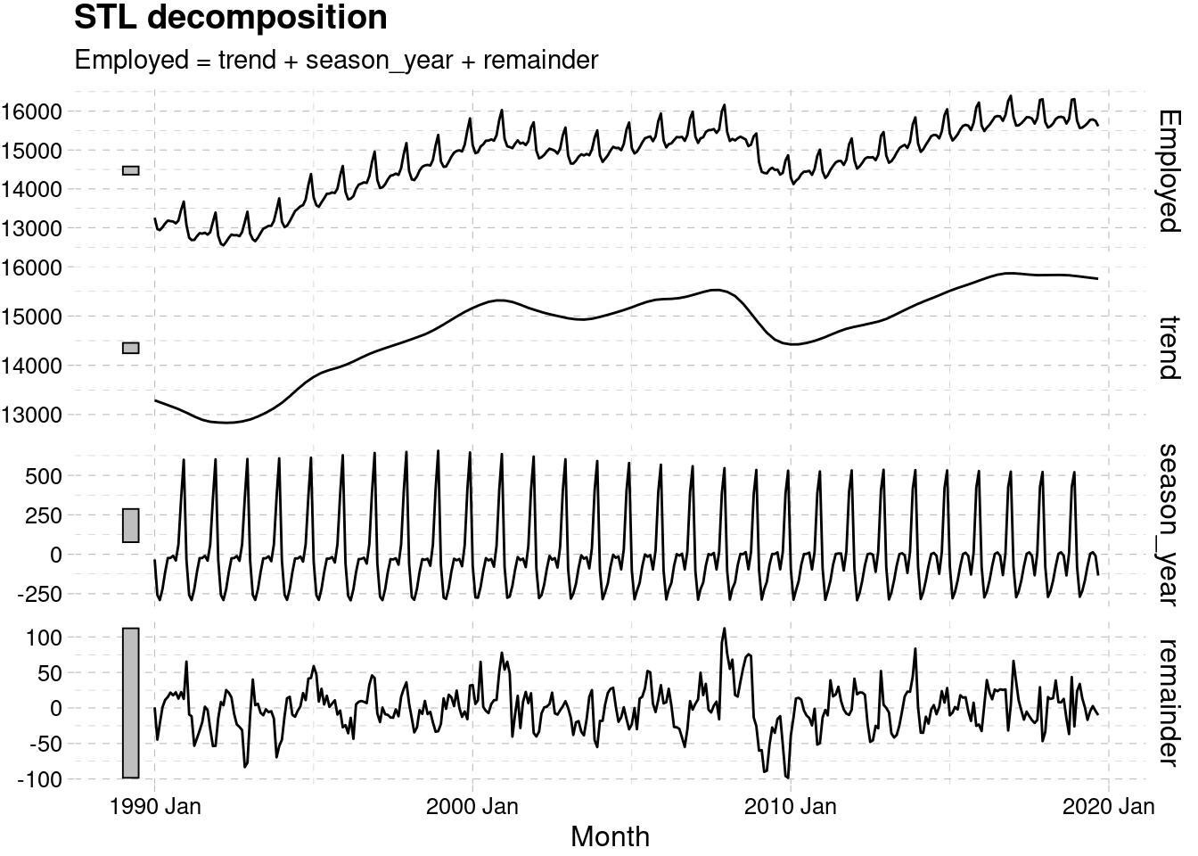
?components
methods("components")## # A tsibble: 6 x 5 [1M]
## Month Employed trend season_adjust remainder
## <mth> <dbl> <dbl> <dbl> <dbl>
## 1 1990 Jan 13256. 13288. 13289. 0.836
## 2 1990 Feb 12966. 13269. 13224. -44.6
## 3 1990 Mar 12938. 13250. 13228. -22.1
## 4 1990 Apr 13012. 13231. 13232. 1.05
## 5 1990 May 13108. 13211. 13223. 11.3
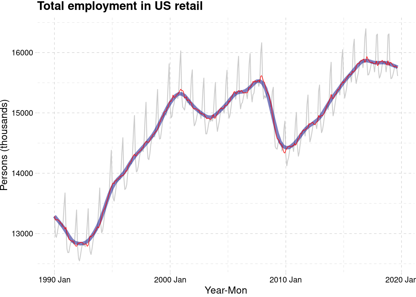
## 6 1990 Jun 13183. 13192. 13207. 15.5components(dcmp) %>%
as_tsibble() %>%
autoplot(Employed, colour="grey80") +
geom_line(aes(y=trend), colour = "navy",linewidth=2,alpha=0.5) +
geom_line(aes(y=season_adjust), colour = "red",linewidth=0.3) +
# geom_line(aes(y=remainder), colour = "blue") +
labs(y = "Persons (thousands)",x="Year-Mon",
title = "Total employment in US retail")+
ggthemes::theme_pander()