8.1 Simple Exponential smoothing
Forecasts produced using exponential smoothing methods are weighted averages of past observations, with the weights decaying exponentially as the observations get older.
Suitable for forecasting data with no clear trend or seasonal pattern
The naïve method assumes that the most recent observation is the only important one, and all previous observations provide no information for the future.
Weighted average \(\hat{y}_{T+h|T}=\frac{1}{T}\sum_{t=1}^T{y_t}\)
With the Exponential smoothing a \(0\leq\alpha\leq1\) is considered as smoothing parameter
- Forecast equation: \(\hat{y}_{t+h|t}=l_t\)
- Smoothing equation: \(l_t=\alpha y_t + (1-\alpha)l_{t-1}\)
\(l_t\) is the smoothed value or the level
\[SSE=\sum_{t=1}^T(y_t-\hat{y}_{t|t-1})^2=\sum_{t=1}^T{e_t^2}\]
\(e_t=y_y-\hat{y}_{t|t-1}\)
library(fpp3)

algeria_economy <- global_economy |>
  filter(Country == "Algeria")


algeria_economy |>
  autoplot(Exports) +
  labs(y = "% of GDP", title = "Exports: Algeria")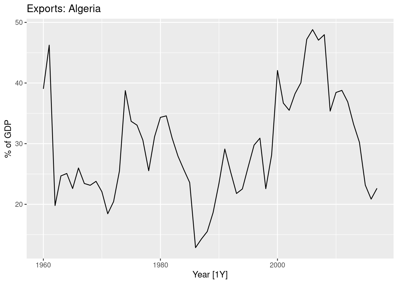
# Estimate parameters
fit <- algeria_economy |>
  model(ETS(Exports ~ error("A") + trend("N") + season("N")))
Parameter estimates
## # A tibble: 2 × 4
##   Country .model                                                  term  estimate
##   <fct>   <chr>                                                   <chr>    <dbl>
## 1 Algeria "ETS(Exports ~ error(\"A\") + trend(\"N\") + season(\"… alpha    0.840
## 2 Algeria "ETS(Exports ~ error(\"A\") + trend(\"N\") + season(\"… l[0]    39.5
tb <- fit%>%augment()
tb[1:59,] %>%
rename(Level=".fitted")%>%
mutate(Time=c(0,seq(1,58,1)),
Year=c(1959,seq(1960,2017,1)),
Observation = lag(Exports),
Forecast=lag(Level))%>%
select(Year,Time,Observation,Level,Forecast)%>%head## # A tibble: 6 × 5
## Year Time Observation Level Forecast
## <dbl> <dbl> <dbl> <dbl> <dbl>
## 1 1959 0 NA 39.5 NA
## 2 1960 1 39.0 39.1 39.5
## 3 1961 2 46.2 45.1 39.1
## 4 1962 3 19.8 23.8 45.1
## 5 1963 4 24.7 24.6 23.8
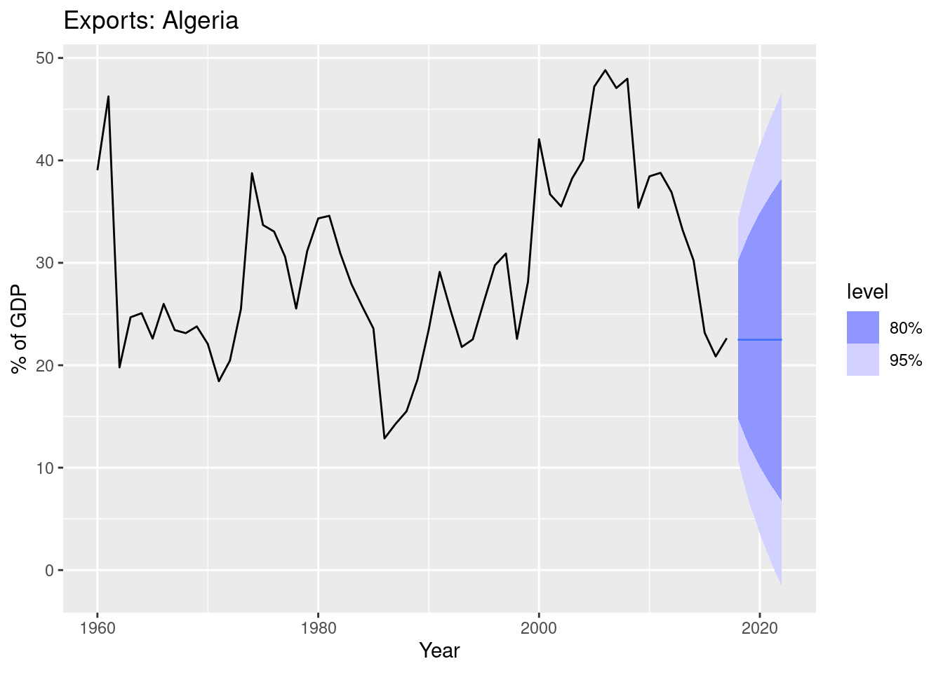
## 6 1964 5 25.1 25.0 24.6fit |>
forecast(h = 5) |>
autoplot(algeria_economy) +
geom_line(aes(y = .fitted), col="#D55E00",
data = augment(fit)) +
labs(y="% of GDP", title="Exports: Algeria") +
guides(colour = "none")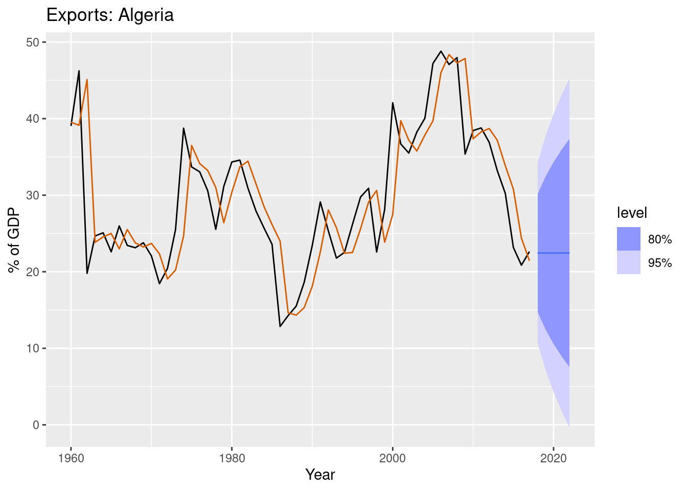
Trend refers to the long-term pattern or direction of a time series. It represents the underlying growth or decline in the data over time. A trend can be upward, downward, or flat, and it can be linear or nonlinear. Trends can be caused by a variety of factors, such as changes in population, technology, or economic conditions.
Seasonality, on the other hand, refers to the pattern of regular fluctuations in a time series that occur at fixed intervals of time, such as daily, weekly, or monthly. Seasonality is often caused by factors such as weather, holidays, or other recurring events. Seasonality can be additive or multiplicative, depending on whether the size of the seasonal fluctuations is constant or varies with the level of the time series.
In summary, trend represents the long-term direction of a time series, while seasonality represents the regular fluctuations that occur at fixed intervals of time. Understanding the trend and seasonality of a time series is important for forecasting and modeling purposes, as it can help to identify the underlying patterns and behavior of the data.
library(purrr)
pred <-
  map2_dfr(fits,
           alpha_range,
           ~ as_tibble(.x %>% augment() %>%
                         mutate(alpha = .y))) %>%
  select(Year,Exports,.fitted,alpha)

pred <- pred %>% as_tibble()library(gganimate)
p <- algeria_economy |>
autoplot(Exports) +
geom_line(aes(y = .fitted,
group=alpha,
col=factor(alpha)),
data =pred) +
transition_states(alpha,
transition_length = 2,
state_length = 1) +
ease_aes('linear')+
labs(y="Exports",color="Alpha") 
## Warning: Removed 1 row containing missing values or values outside the scale range
## (`geom_line()`).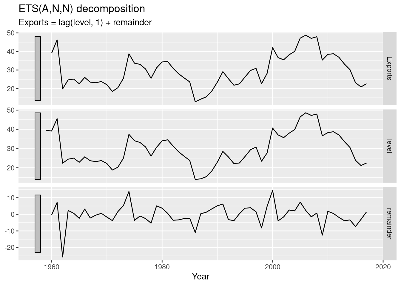
## # A dable: 6 x 7 [1Y]
## # Key:     Country, .model [1]
## # :        Exports = lag(level, 1) + remainder
##   Country .model                            Year Exports level remainder .fitted
##   <fct>   <chr>                            <dbl>   <dbl> <dbl>     <dbl>   <dbl>
## 1 Algeria "ETS(Exports ~ error(\"A\") + t…  1959    NA    39.5    NA        NA
## 2 Algeria "ETS(Exports ~ error(\"A\") + t…  1960    39.0  39.1    -0.465    39.5
## 3 Algeria "ETS(Exports ~ error(\"A\") + t…  1961    46.2  45.5     7.15     39.1
## 4 Algeria "ETS(Exports ~ error(\"A\") + t…  1962    19.8  22.4   -25.7      45.5
## 5 Algeria "ETS(Exports ~ error(\"A\") + t…  1963    24.7  24.5     2.32     22.4
## 6 Algeria "ETS(Exports ~ error(\"A\") + t…  1964    25.1  25.0     0.631    24.5