3.4 Methods used by official statistics agencies

US Census Bureau, Australian Bureau of Statistics and other official statistics agencies have developed their own decomposition procedures which are used for seasonal adjustment.

3.4.1 X-11 method

It requires the seasonal package.

x11_dcmp <- us_retail_employment %>%
  model(x11 = X_13ARIMA_SEATS(Employed ~ x11())) %>%
  components()


autoplot(x11_dcmp) +
  labs(title =
    "Decomposition of total US retail employment using X-11.")+
  ggthemes::theme_pander()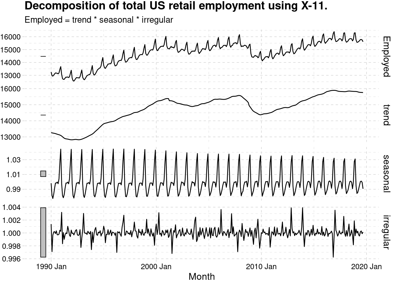

The X-11 trend-cycle has captured the sudden fall in the data due to the 2007–2008 global financial crisis better than either of the other two methods.

x11_dcmp %>%
  ggplot(aes(x = Month)) +
  geom_line(aes(y = Employed, colour = "Data")) +
  geom_line(aes(y = season_adjust,
                colour = "Seasonally Adjusted")) +
  geom_line(aes(y = trend, colour = "Trend")) +
  labs(y = "Persons (thousands)",
       title = "Total employment in US retail") +
  scale_colour_manual(
    values = c("gray", "#0072B2", "#D55E00"),
    breaks = c("Data", "Seasonally Adjusted", "Trend")
  )+
  ggthemes::theme_pander()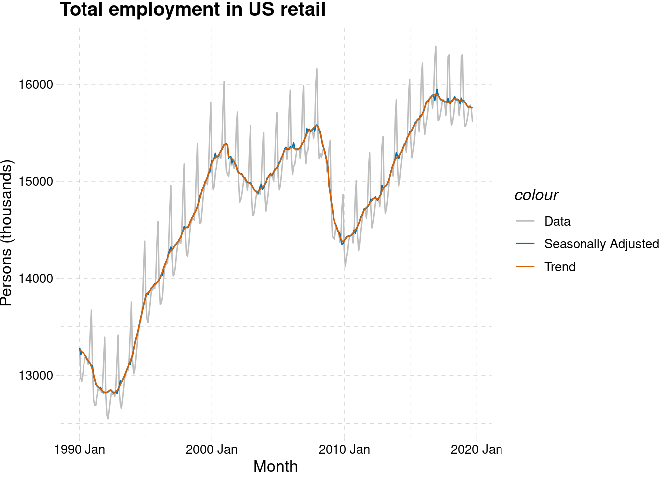

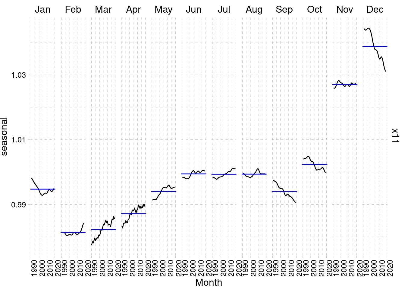
To help us visualise the variation in the seasonal component over time

x11_dcmp %>%
  gg_subseries(seasonal)+
  ggthemes::theme_pander()

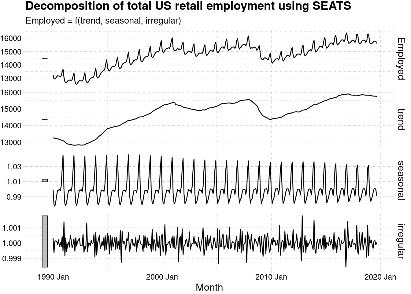
3.4.2 The SEATS method

The SEATS: Seasonal Extraction in ARIMA Time Series developed at the Bank of Spain

seats_dcmp <- us_retail_employment %>%
  model(seats = X_13ARIMA_SEATS(Employed ~ seats())) %>%
  components()


autoplot(seats_dcmp) +
  labs(title =
    "Decomposition of total US retail employment using SEATS")+
  ggthemes::theme_pander()