5.1 EXRCISE 1
Produce forecasts for the following series using whichever of NAIVE(y), SNAIVE(y) or RW(y ~ drift()) is more appropriate in each case:
- Australian Population (global_economy)
- Bricks (aus_production)
- NSW Lambs (aus_livestock)
- Household wealth (hh_budget)
- Australian takeaway food turnover (aus_retail)
5.1.1 Australian Population (global_economy)
data(global_economy)

df <- global_economy %>%
  filter(Country=="Australia") %>%
  mutate(GDP_pop=GDP/Population)

df%>%head
## # A tsibble: 6 x 10 [1Y]
## # Key: Country [1]
## Country Code Year GDP Growth CPI Imports Exports Population GDP_pop
## <fct> <fct> <dbl> <dbl> <dbl> <dbl> <dbl> <dbl> <dbl> <dbl>
## 1 Australia AUS 1960 1.86e10 NA 7.96 14.1 13.0 10276477 1807.
## 2 Australia AUS 1961 1.96e10 2.49 8.14 15.0 12.4 10483000 1874.
## 3 Australia AUS 1962 1.99e10 1.30 8.12 12.6 13.9 10742000 1851.
## 4 Australia AUS 1963 2.15e10 6.21 8.17 13.8 13.0 10950000 1964.
## 5 Australia AUS 1964 2.38e10 6.98 8.40 13.8 14.9 11167000 2128.
## 6 Australia AUS 1965 2.59e10 5.98 8.69 15.3 13.2 11388000 2277.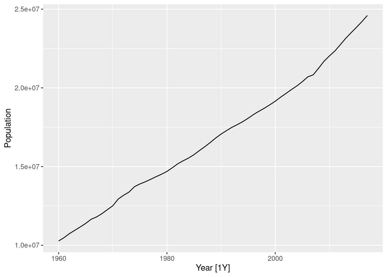
df %>%
  select(Population,GDP_pop)%>%
  scale()%>%
  as_data_frame()%>%
  cbind(Year2=df$Year)%>%
  ggplot(aes(Year2,Population))+
  geom_point(shape=21,stroke=0.5)+
  geom_line()+
  geom_smooth(method = 'loess', se = FALSE, color = 'red',linewidth=0.3) +
  geom_line(aes(Year2,GDP_pop))+
  scale_x_continuous(n.breaks = 10)+
  geom_text(aes(x=c(1990), y=c(0.5), label="Pop"),color="red")+
  geom_text(aes(x=c(2005), y=c(2.5), label="GDP/Pop"))+
  labs(title="Australian Population and GDP/Population")+
  theme_bw()
## Warning: `as_data_frame()` was deprecated in tibble 2.0.0.
## ℹ Please use `as_tibble()` (with slightly different semantics) to convert to a
## tibble, or `as.data.frame()` to convert to a data frame.
## This warning is displayed once every 8 hours.
## Call `lifecycle::last_lifecycle_warnings()` to see where this warning was
## generated.## Warning in geom_text(aes(x = c(1990), y = c(0.5), label = "Pop"), color = "red"): All aesthetics have length 1, but the data has 58 rows.
## ℹ Did you mean to use `annotate()`?## Warning in geom_text(aes(x = c(2005), y = c(2.5), label = "GDP/Pop")): All aesthetics have length 1, but the data has 58 rows.
## ℹ Did you mean to use `annotate()`?## `geom_smooth()` using formula = 'y ~ x'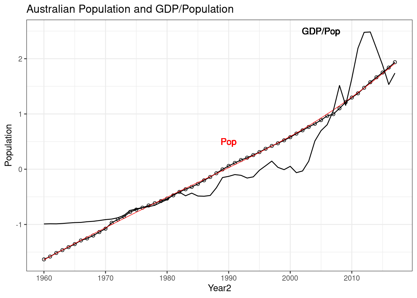
df %>%
  model(
    `Naïve` = NAIVE(Population),
    `Seasonal naïve` = SNAIVE(Population),
    Drift = RW(log(Population) ~ drift())
  ) %>%
    forecast(h = c(10,20)) %>%
    autoplot(df |> filter(!is.na(Population)),
    point_forecast = lst(mean, median)
  )
## Warning: 1 error encountered for Seasonal naïve
## [1] Non-seasonal model specification provided, use RW() or provide a different lag specification.## Warning: There were 3 warnings in `mutate()`.
## The first warning was:
## ℹ In argument: `Naïve = (function (object, ...) ...`.
## Caused by warning:
## ! More than one forecast horizon specified, using the smallest.
## ℹ Run `dplyr::last_dplyr_warnings()` to see the 2 remaining warnings.## Warning in max(ids, na.rm = TRUE): no non-missing arguments to max; returning
## -Inf
## Warning in max(ids, na.rm = TRUE): no non-missing arguments to max; returning
## -Inf## Warning: Removed 20 rows containing missing values or values outside the scale range
## (`geom_line()`).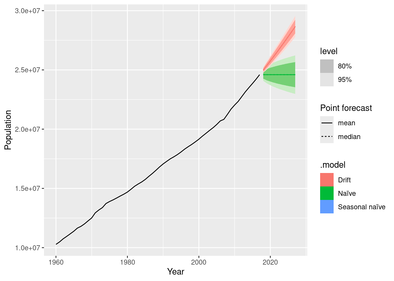
## Warning: Removed 1 row containing missing values or values outside the scale range
## (`geom_line()`).
## Warning: Removed 1 row containing missing values or values outside the scale range
## (`geom_point()`).## Warning: Removed 1 row containing non-finite outside the scale range
## (`stat_bin()`).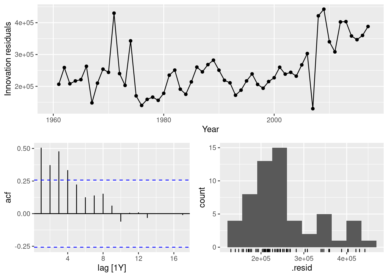
fit_pop_drift <- df %>%
  model(Drift = RW(log(Population) ~ drift()))


fit_pop_drift |> gg_tsresiduals()
## Warning: Removed 1 row containing missing values or values outside the scale range
## (`geom_line()`).## Warning: Removed 1 row containing missing values or values outside the scale range
## (`geom_point()`).## Warning: Removed 1 row containing non-finite outside the scale range
## (`stat_bin()`).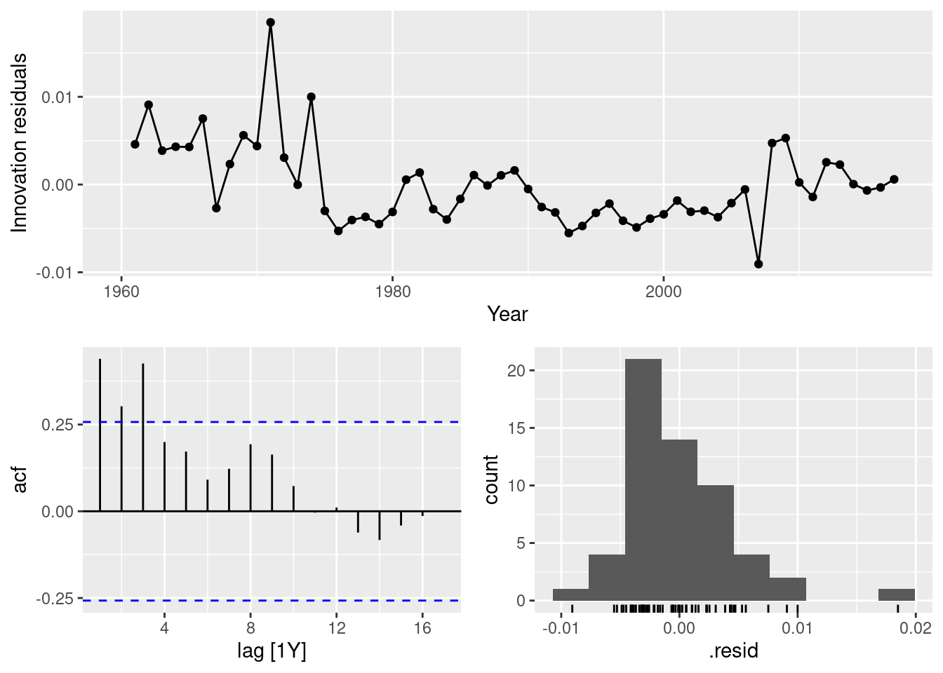
5.1.2 Bricks (aus_production)
## # A tsibble: 6 x 7 [1Q]
##   Quarter  Beer Tobacco Bricks Cement Electricity   Gas
##     <qtr> <dbl>   <dbl>  <dbl>  <dbl>       <dbl> <dbl>
## 1 1956 Q1   284    5225    189    465        3923     5
## 2 1956 Q2   213    5178    204    532        4436     6
## 3 1956 Q3   227    5297    208    561        4806     7
## 4 1956 Q4   308    5681    197    570        4418     6
## 5 1957 Q1   262    5577    187    529        4339     5
## 6 1957 Q2 228 5651 214 604 4811 7## Warning: Removed 20 rows containing missing values or values outside the scale range
## (`geom_line()`).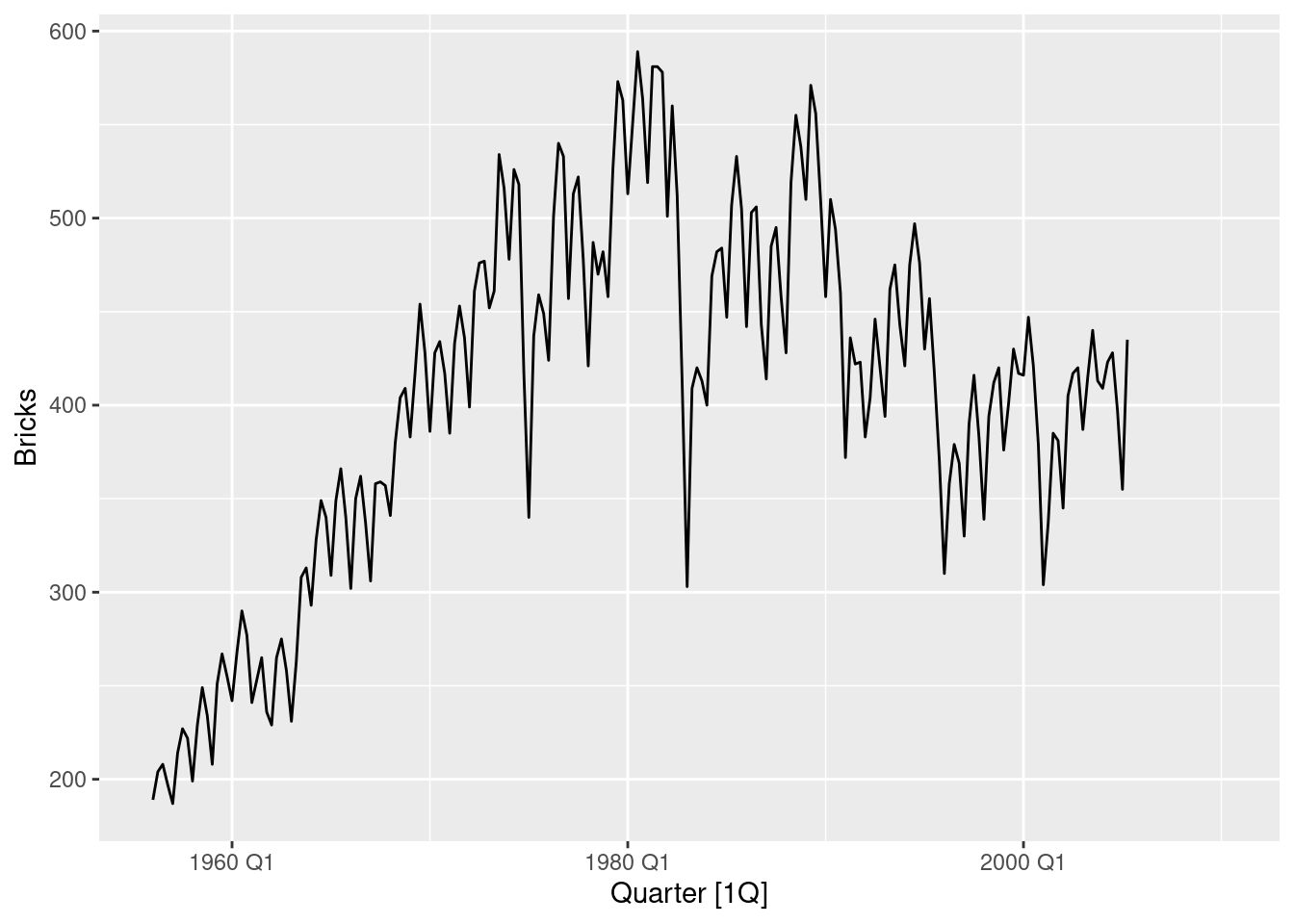
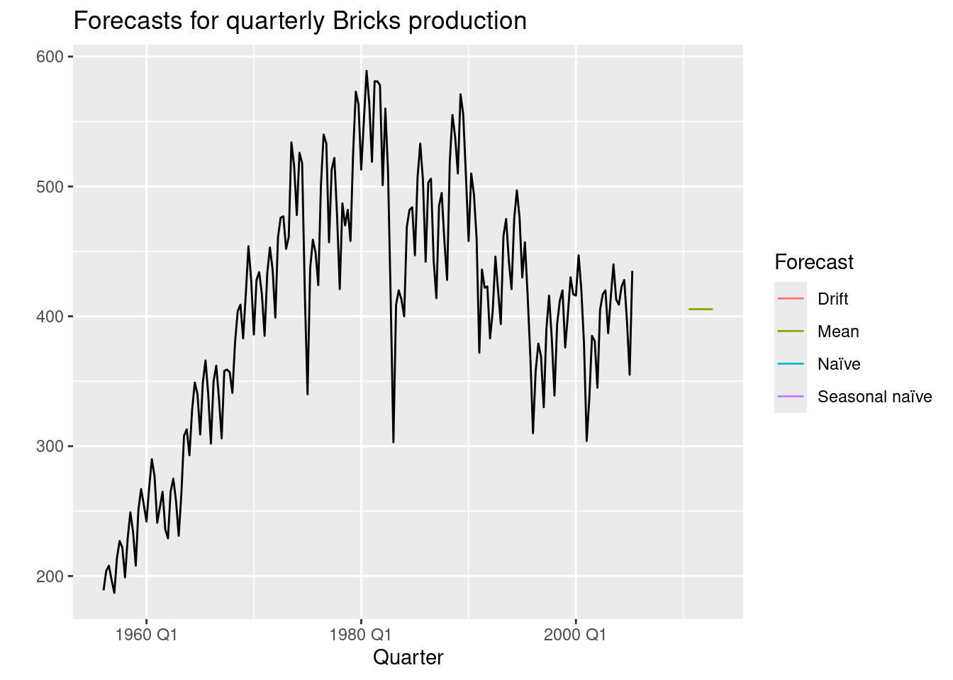
bricks_fit <- aus_production |>
  model(
    Mean = MEAN(Bricks),
    `Naïve` = NAIVE(Bricks),
    `Seasonal naïve` = SNAIVE(Bricks),
    Drift = RW(Bricks ~ drift())
  )

bricks_fc <- bricks_fit |>
  forecast(h = 10)

bricks_fc |>
  autoplot(
    aus_production,
    level = NULL
  ) +
  labs(
    y = "",
    title = "Forecasts for quarterly Bricks production"
  ) +
  guides(colour = guide_legend(title = "Forecast"))
## Warning: Removed 30 rows containing missing values or values outside the scale range
## (`geom_line()`).## Warning: Removed 20 rows containing missing values or values outside the scale range
## (`geom_line()`).