12.1 Complex seasonality
Daily data:
- weekly pattern (365.25/7 \(\approx\) 52.179 on average)
- annual pattern
Hourly data:
- daily pattern
- weekly pattern
- annual pattern
12.1.1 Case Study 1
Number of calls (call volume) to a North American commercial bank per 5-minute interval between 7:00am and 9:05pm each weekday over a 33 week period.
In this case we have a weak daily and weekly seasonal patterns:
- on a total of
164 daysfrom March 03, 2003 to Oct 24, 2003. - there are
169 5-minute intervals per day: \[169×5=845\] - a total of
845 minutes per day(5-days a week) spent on bank calls.
Let’s have a look at the seasonality per day and per week.
## # A tsibble: 6 x 2 [5m] <UTC>
##   DateTime            Calls
##   <dttm>              <dbl>
## 1 2003-03-03 07:00:00   111
## 2 2003-03-03 07:05:00   113
## 3 2003-03-03 07:10:00    76
## 4 2003-03-03 07:15:00    82
## 5 2003-03-03 07:20:00    91
## 6 2003-03-03 07:25:00 87## # A tsibble: 6 x 2 [5m] <UTC>
## DateTime Calls
## <dttm> <dbl>
## 1 2003-10-24 20:35:00 56
## 2 2003-10-24 20:40:00 64
## 3 2003-10-24 20:45:00 49
## 4 2003-10-24 20:50:00 54
## 5 2003-10-24 20:55:00 55
## 6 2003-10-24 21:00:00 54## # A tibble: 6 × 2
## date n
## <date> <int>
## 1 2003-03-03 169
## 2 2003-03-04 169
## 3 2003-03-05 169
## 4 2003-03-06 169
## 5 2003-03-07 169
## 6 2003-03-10 169per_day <- bank_calls%>%
mutate(date=as.Date(DateTime))%>%
group_by(date)%>%
reframe(tot_calls=sum(Calls))
per_day%>%dim## [1] 164 2We cannot see a clear pattern for seasonality here.
## `geom_smooth()` using method = 'loess' and formula = 'y ~ x'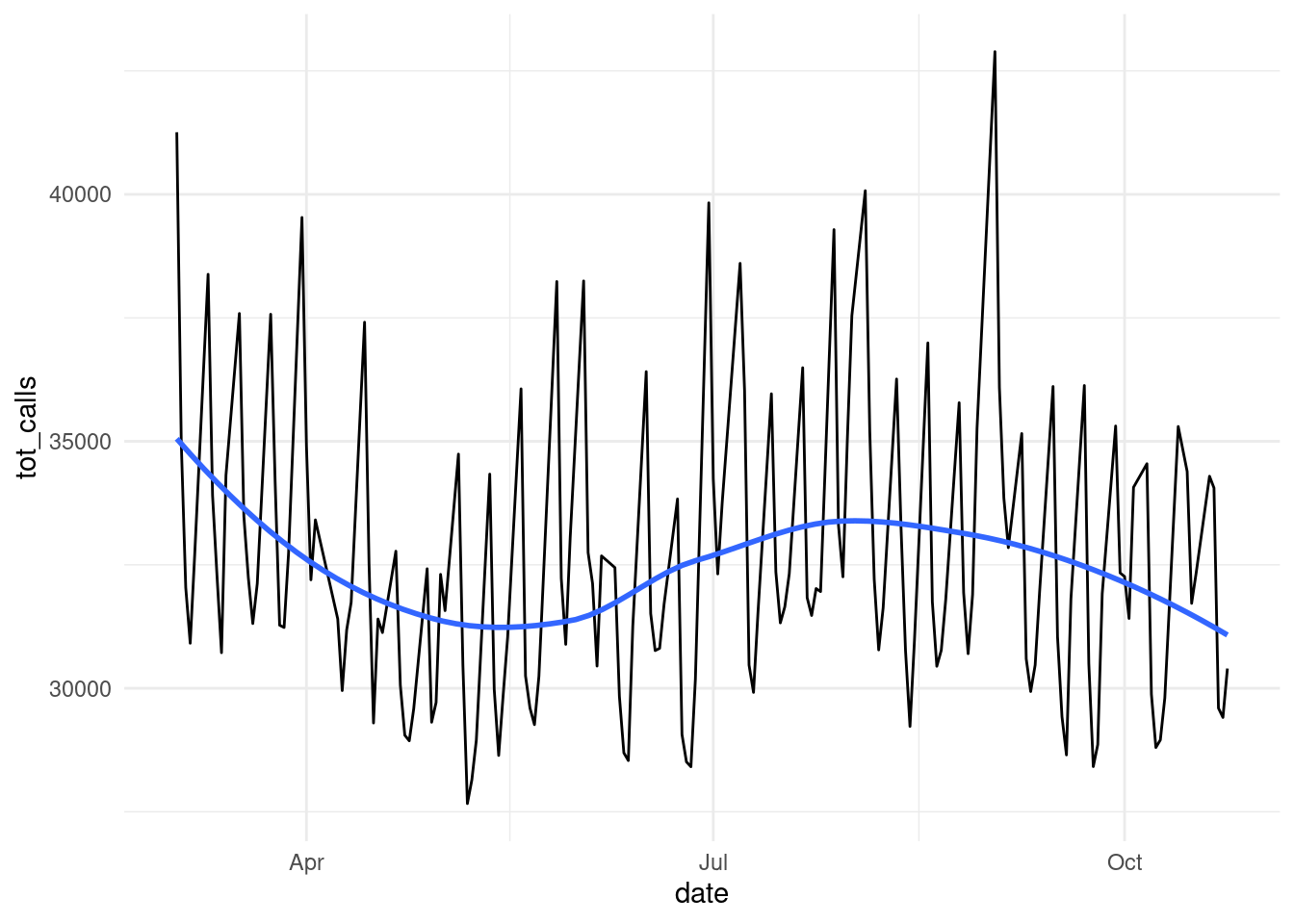
bank_calls |>
  fill_gaps() |>
  autoplot(Calls) +
  labs(y = "Calls",
       title = "Five-minute call volume to bank")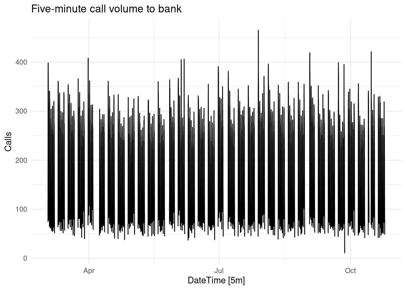
bank_calls |>
  fill_gaps() %>%
  mutate(month=month(DateTime),
         day=day(DateTime),
         week=week(DateTime))%>%
  filter(month<4)%>%
  ggplot(aes(x=DateTime,y=Calls,group=week))+
  geom_line()
## Warning: Removed 511 rows containing missing values or values outside the scale range
## (`geom_line()`).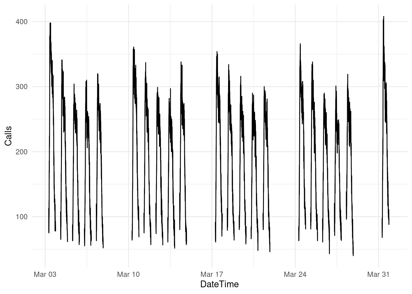
Have a look at multiple seasonality with the STL() decomposition:
calls <- bank_calls |>
  mutate(t = row_number()) |>
  update_tsibble(index = t, regular = TRUE)
calls%>%head
## # A tsibble: 6 x 3 [1]
## DateTime Calls t
## <dttm> <dbl> <int>
## 1 2003-03-03 07:00:00 111 1
## 2 2003-03-03 07:05:00 113 2
## 3 2003-03-03 07:10:00 76 3
## 4 2003-03-03 07:15:00 82 4
## 5 2003-03-03 07:20:00 91 5
## 6 2003-03-03 07:25:00 87 6calls |>
model(
STL(sqrt(Calls) ~ season(period = 169) +
season(period = 5*169),
robust = TRUE)
) |>
components() |>
select(t,season_169,season_845) %>%
pivot_longer(cols = c("season_169","season_845"))%>%
ggplot(aes(x=t,y=value)) +
geom_line()+
facet_wrap(vars(name),ncol = 1,scales = "free")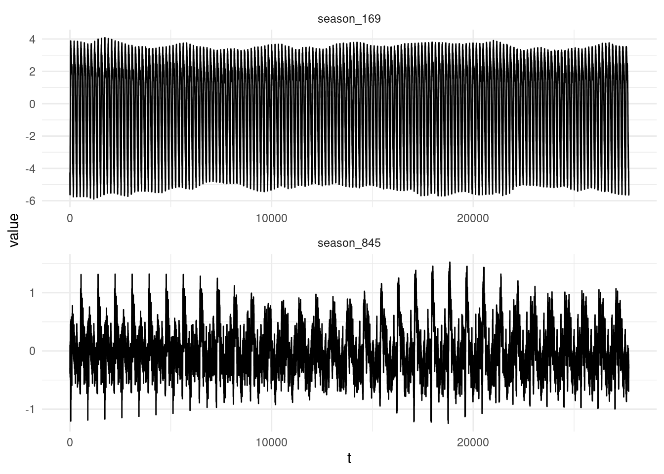
Decomposition used in forecasting:
# Forecasts from STL+ETS decomposition
my_dcmp_spec <- decomposition_model(
  STL(sqrt(Calls) ~ season(period = 169) +
                    season(period = 5*169),
      robust = TRUE),
  # ETS decomposition
  ETS(season_adjust ~ season("N"))
  )
Forecast 5*169 forward
## # A fable: 6 x 4 [1]
## # Key:     .model [1]
##   .model           t           Calls .mean
##   <chr>        <dbl>          <dist> <dbl>
## 1 my_dcmp_spec 27717 t(N(8.8, 0.24))  76.8
## 2 my_dcmp_spec 27718 t(N(9.2, 0.25))  85.7
## 3 my_dcmp_spec 27719 t(N(8.9, 0.25))  79.8
## 4 my_dcmp_spec 27720 t(N(8.6, 0.26))  75.0
## 5 my_dcmp_spec 27721 t(N(9.2, 0.27))  85.0
## 6 my_dcmp_spec 27722 t(N(8.7, 0.28))  75.7
# Add correct time stamps to fable
fc_with_times <- bank_calls |>
new_data(n = 7 * 24 * 60 / 5) |>
mutate(time = format(DateTime, format = "%H:%M:%S")) |>
filter(
time %in% format(bank_calls$DateTime, format = "%H:%M:%S"),
wday(DateTime, week_start = 1) <= 5
) |>
mutate(t = row_number() + max(calls$t)) |>
left_join(fc, by = "t") |>
as_fable(response = "Calls", distribution = Calls)
fc_with_times%>%head()## # A fable: 6 x 6 [5m] <UTC>
## DateTime time t .model Calls .mean
## <dttm> <chr> <dbl> <chr> <dist> <dbl>
## 1 2003-10-27 07:00:00 07:00:00 27717 my_dcmp_spec t(N(8.8, 0.24)) 76.8
## 2 2003-10-27 07:05:00 07:05:00 27718 my_dcmp_spec t(N(9.2, 0.25)) 85.7
## 3 2003-10-27 07:10:00 07:10:00 27719 my_dcmp_spec t(N(8.9, 0.25)) 79.8
## 4 2003-10-27 07:15:00 07:15:00 27720 my_dcmp_spec t(N(8.6, 0.26)) 75.0
## 5 2003-10-27 07:20:00 07:20:00 27721 my_dcmp_spec t(N(9.2, 0.27)) 85.0
## 6 2003-10-27 07:25:00 07:25:00 27722 my_dcmp_spec t(N(8.7, 0.28)) 75.7# Plot results with last 3 weeks of data
fc_with_times |>
fill_gaps() |>
autoplot(bank_calls |> tail(14 * 169) |> fill_gaps()) +
labs(y = "Calls",
title = "Five-minute call volume to bank")## Warning: Removed 100 rows containing missing values or values outside the scale range
## (`geom_line()`).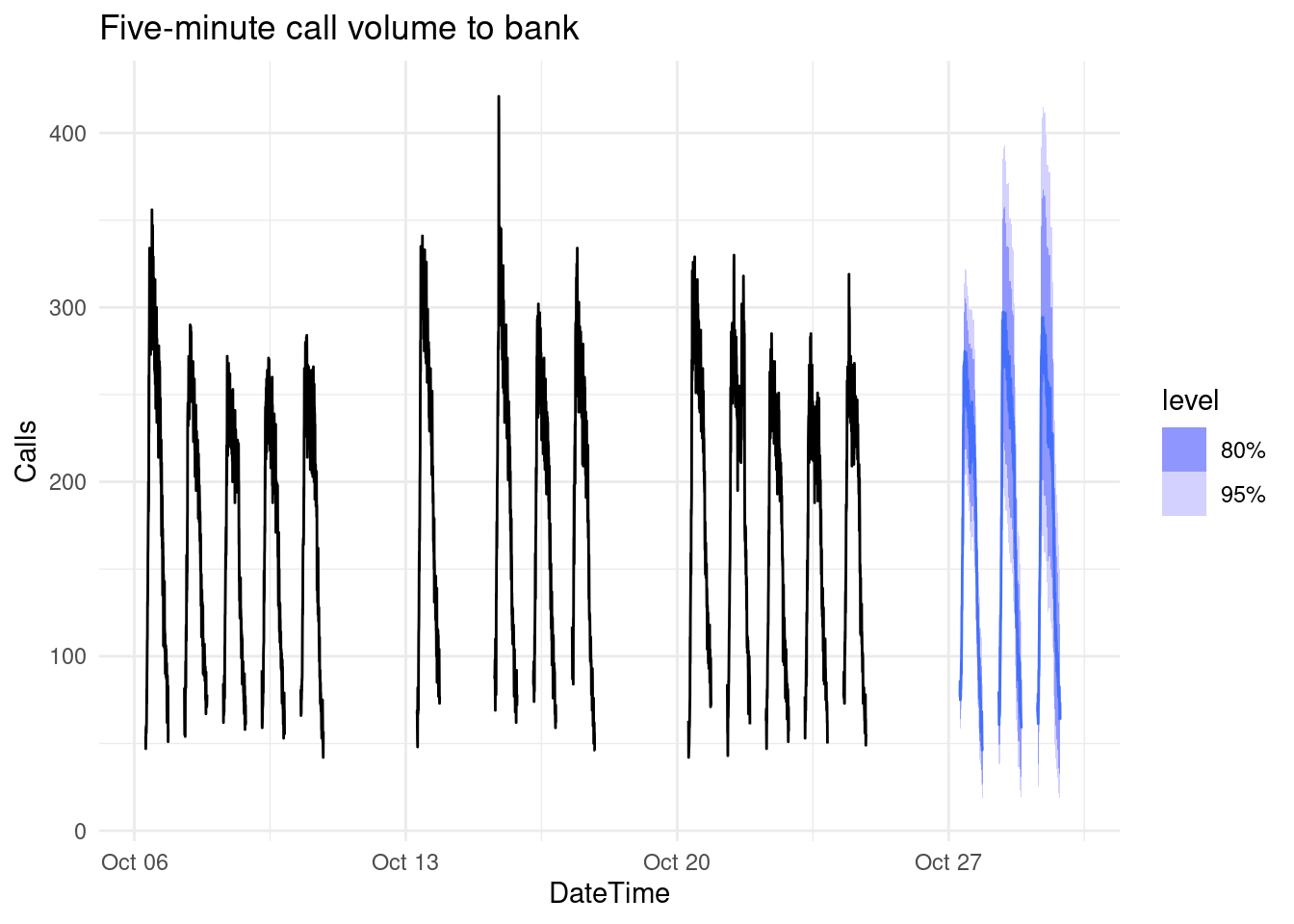
Apply Fourier for multiple seasonalities: fit a dynamic harmonic regression model with an ARIMA error structure.
fit <- calls |>
  model(
    dhr = ARIMA(sqrt(Calls) ~ PDQ(0, 0, 0) + pdq(d = 0) +
                  fourier(period = 169, K = 10) +
fourier(period = 5*169, K = 5)))# Add correct time stamps to fable
fc_with_times <- bank_calls |>
new_data(n = 7 * 24 * 60 / 5) |>
mutate(time = format(DateTime,
format = "%H:%M:%S")) |>
filter(
time %in% format(bank_calls$DateTime,
format = "%H:%M:%S"),
wday(DateTime, week_start = 1) <= 5
) |>
mutate(t = row_number() + max(calls$t)) |>
left_join(fc, by = "t") |>
as_fable(response = "Calls", distribution = Calls)12.1.2 Case Study 2
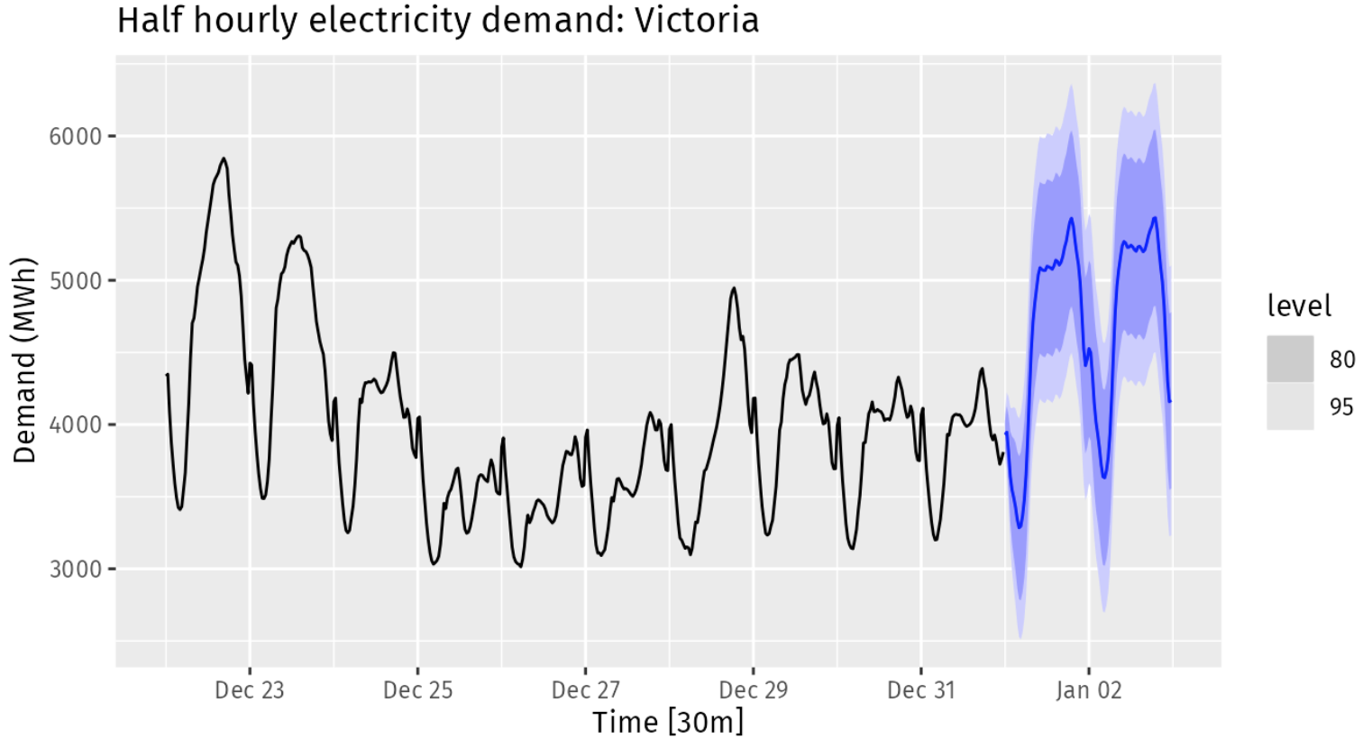
Electricity demand (MWh) in Victoria, Australia, during 2012–2014 (half-hourly) along with temperatures (degrees Celsius) for the same period for Melbourne.
## # A tsibble: 6 x 5 [30m] <Australia/Melbourne>
##   Time                Demand Temperature Date       Holiday
##   <dttm>               <dbl>       <dbl> <date>     <lgl>
## 1 2012-01-01 00:00:00  4383.        21.4 2012-01-01 TRUE
## 2 2012-01-01 00:30:00  4263.        21.0 2012-01-01 TRUE
## 3 2012-01-01 01:00:00  4049.        20.7 2012-01-01 TRUE
## 4 2012-01-01 01:30:00  3878.        20.6 2012-01-01 TRUE
## 5 2012-01-01 02:00:00  4036.        20.4 2012-01-01 TRUE
## 6 2012-01-01 02:30:00  3866.        20.2 2012-01-01 TRUE
vic_elec |>
pivot_longer(Demand:Temperature, names_to = "Series") |>
ggplot(aes(x = Time, y = value)) +
geom_line() +
facet_grid(rows = vars(Series), scales = "free_y") +
labs(y = "")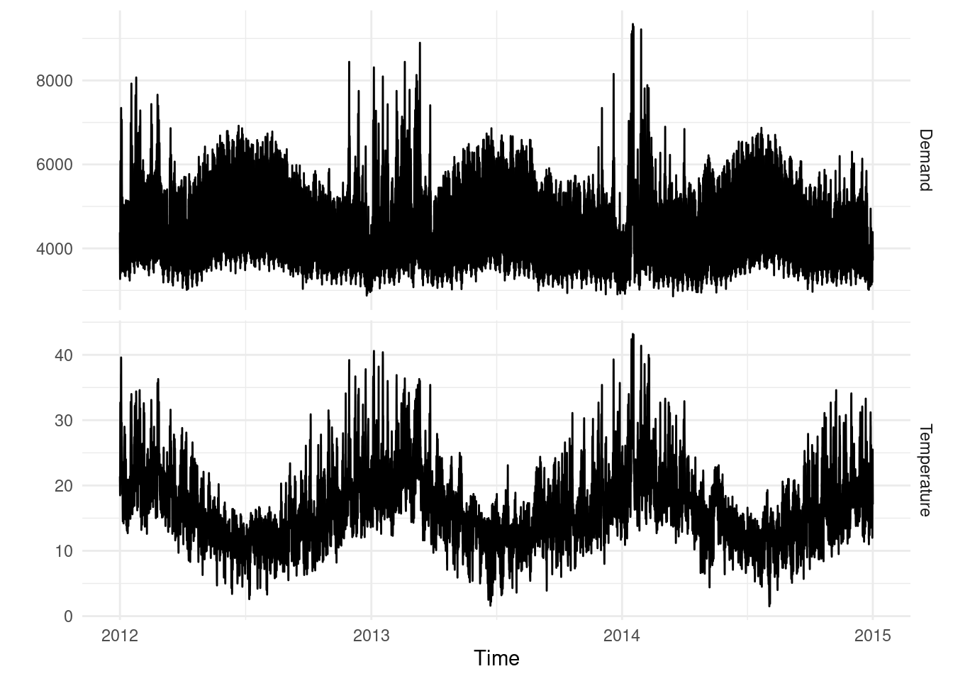
elec <- vic_elec |>
  mutate(
    DOW = wday(Date, label = TRUE),
    Working_Day = !Holiday & !(DOW %in% c("Sat", "Sun")),
    Cooling = pmax(Temperature, 18)
  )

elec%>%head
## # A tsibble: 6 x 8 [30m] <Australia/Melbourne>
## Time Demand Temperature Date Holiday DOW Working_Day
## <dttm> <dbl> <dbl> <date> <lgl> <ord> <lgl>
## 1 2012-01-01 00:00:00 4383. 21.4 2012-01-01 TRUE Sun FALSE
## 2 2012-01-01 00:30:00 4263. 21.0 2012-01-01 TRUE Sun FALSE
## 3 2012-01-01 01:00:00 4049. 20.7 2012-01-01 TRUE Sun FALSE
## 4 2012-01-01 01:30:00 3878. 20.6 2012-01-01 TRUE Sun FALSE
## 5 2012-01-01 02:00:00 4036. 20.4 2012-01-01 TRUE Sun FALSE
## 6 2012-01-01 02:30:00 3866. 20.2 2012-01-01 TRUE Sun FALSE
## # ℹ 1 more variable: Cooling <dbl>elec |>
ggplot(aes(x=Temperature, y=Demand, col=Working_Day)) +
geom_point(alpha = 0.6) +
labs(x="Temperature (degrees Celsius)", y="Demand (MWh)")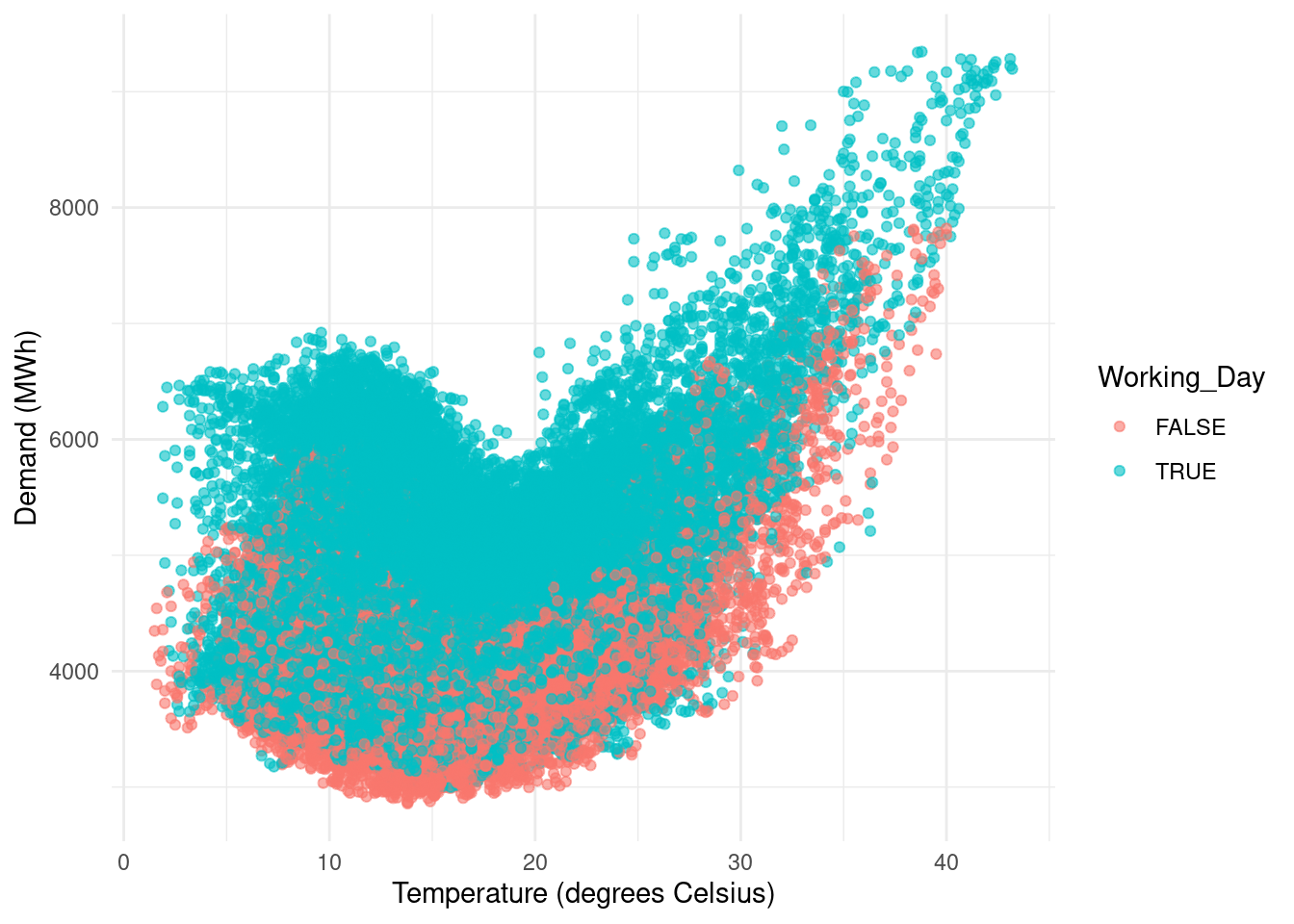
fit2 <- elec |>
  model(
    ARIMA(Demand ~ PDQ(0, 0, 0) + pdq(d = 0) +
          Temperature + Cooling + Working_Day +
          fourier(period = "day", K = 10) +
          fourier(period = "week", K = 5) +
          fourier(period = "year", K = 3))
  )
new_data:
elec_newdata <- new_data(elec, 2*48) |>
  mutate(
    Temperature = tail(elec$Temperature, 2 * 48),
    Date = lubridate::as_date(Time),
    DOW = wday(Date, label = TRUE),
    Working_Day = (Date != "2015-01-01") &
                   !(DOW %in% c("Sat", "Sun")),
    Cooling = pmax(Temperature, 18)
  )
fc |>
autoplot(elec |> tail(10 * 48)) +
labs(title="Half hourly electricity demand: Victoria",
y = "Demand (MWh)", x = "Time [30m]")