10.3 Example: US Personal Consumption and Income

Forecast changes in expenditure based on changes in income. In this case data are already stationary, and there is no need for any differencing.

library(tidyverse)
library(fpp3)
us_change |>
  pivot_longer(c(Consumption, Income),
               names_to = "var", values_to = "value") |>
  ggplot(aes(x = Quarter, y = value)) +
  geom_line() +
  facet_grid(vars(var), scales = "free_y") +
  labs(title = "US consumption and personal income",
       y = "Quarterly % change")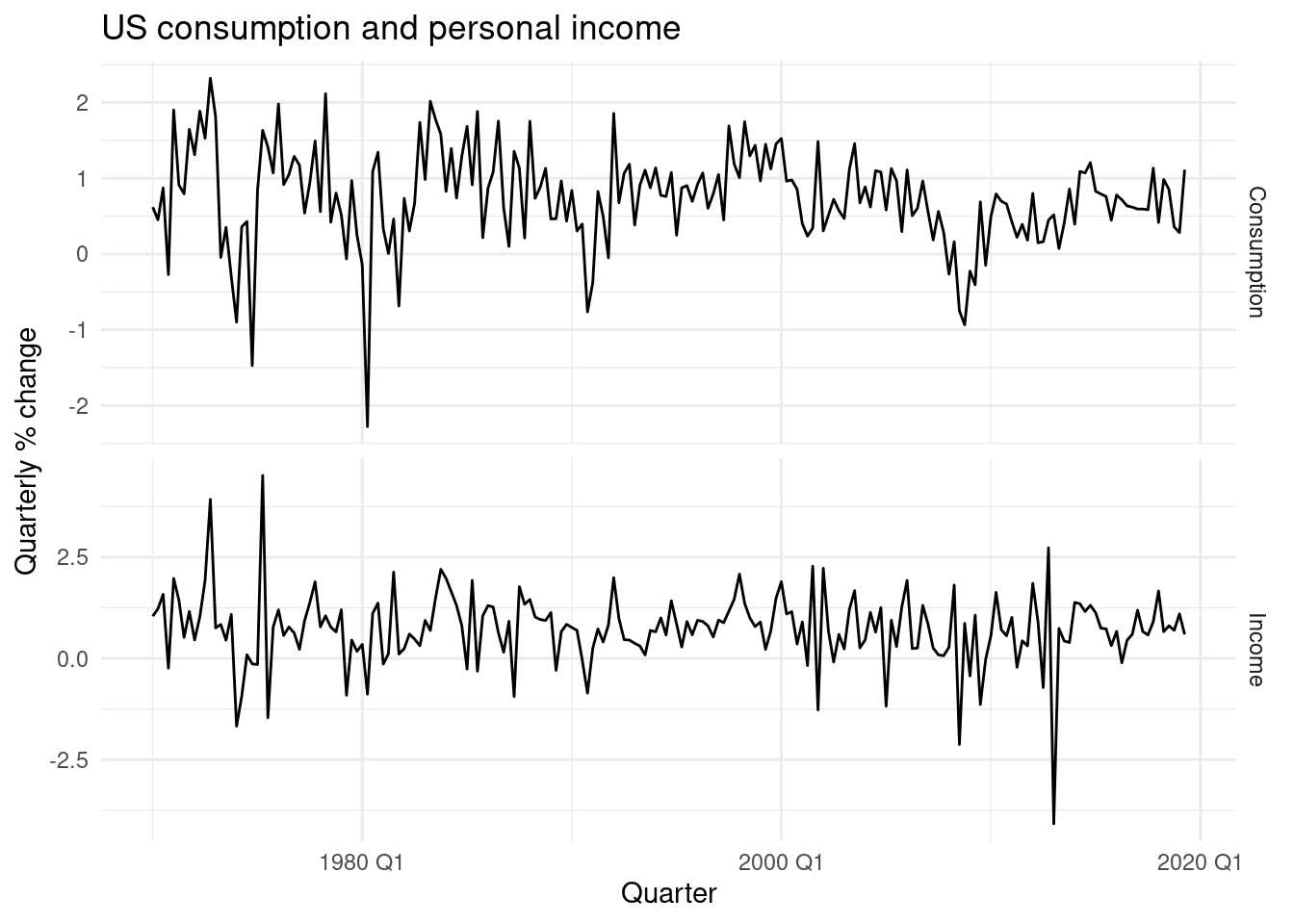

fit <- us_change |>
  model(ARIMA(Consumption ~ Income))
report(fit)

## Series: Consumption 
## Model: LM w/ ARIMA(1,0,2) errors 
## 
## Coefficients:
##          ar1      ma1     ma2  Income  intercept
##       0.7070  -0.6172  0.2066  0.1976     0.5949
## s.e.  0.1068   0.1218  0.0741  0.0462     0.0850
## 
## sigma^2 estimated as 0.3113:  log likelihood=-163.04
## AIC=338.07   AICc=338.51   BIC=357.8

The model relases this ARIMA model selection: $$ARIMA(1,0,2) \text{ ; errors}$$

$$y_t=0.595+0.198x_t+ \eta_t$$ $$\eta_t=0.707 \eta_{t-1}+\varepsilon_t - 0.617 \varepsilon_{t-1}+ 0.207\varepsilon_{t-2}$$ $$\varepsilon_t \sim NID(0,0.311)$$

The residual() function applied on the model fit release the estimates for both:

• $\eta_t$
• $\varepsilon_t$

bind_rows(
    `Regression residuals` =
        as_tibble(residuals(fit, type = "regression")),
    `ARIMA residuals` =
        as_tibble(residuals(fit, type = "innovation")),
    .id = "type"
  ) |>
  mutate(
    type = factor(type, levels=c(
      "Regression residuals", "ARIMA residuals"))
  ) |>
  ggplot(aes(x = Quarter, y = .resid)) +
  geom_line() +
  facet_grid(vars(type))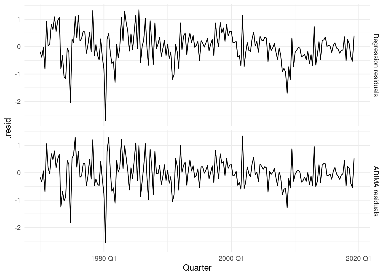

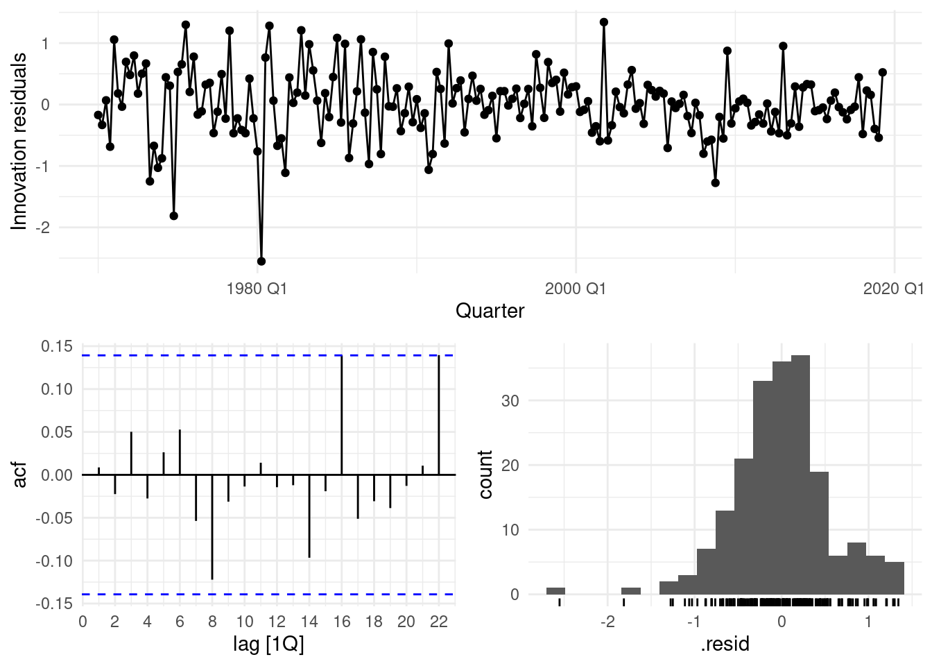
fit |> gg_tsresiduals()

augment(fit) |>
  features(.innov, ljung_box, dof = 3, lag = 8)

## # A tibble: 1 × 3
##   .model                      lb_stat lb_pvalue
##   <chr>                         <dbl>     <dbl>
## 1 ARIMA(Consumption ~ Income)    5.21     0.391