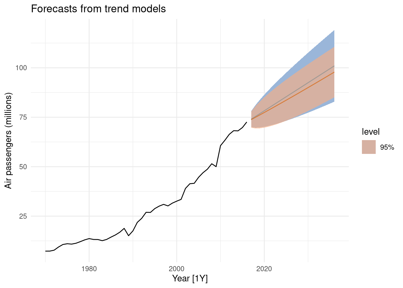
10.5 Difference between Stochastic and deterministic trends

$$y_t=\beta_0+\beta_1x+\eta_t$$

• Deterministic $\eta_t \sim ARIMA(p,0,q)$
• Stochastic $\eta_t \sim ARIMA(p,1,q)$

fit_deterministic <- aus_airpassengers |>
  model(deterministic = ARIMA(Passengers ~ 1 + trend() +
                                pdq(d = 0)))

fit_stochastic <- aus_airpassengers |>
  model(stochastic = ARIMA(Passengers ~ pdq(d = 1)))

## Scale for fill_ramp is already present.
## Adding another scale for fill_ramp, which will replace the existing scale.