7.4 Least squares estimation

“fitting” the model to the data, or sometimes “learning” or “training” the model.

“The least squares principle provides a way of choosing the coefficients effectively by minimizing the sum of the squared errors.” The Author

Formula: \(\sum_{t=1}^T{\epsilon_t^2}=\sum_{t=1}^T{(y_t-\beta_0+\beta_1x_{1,t}+\beta_2x_{2,t}+...+\beta_kx_{k,t}+\epsilon_t)^2}\)

\[\sum{\epsilon^2}=\sum{(Y-\beta X)^2}\]

fit_consMR <- us_change |>
  model(tslm = TSLM(Consumption ~ Income + Production +
                                    Unemployment + Savings))

augment(fit_consMR)[3:5]%>%head

## # A tibble: 6 × 3
##   Consumption .fitted  .resid
##         <dbl>   <dbl>   <dbl>
## 1       0.619   0.474  0.145 
## 2       0.452   0.635 -0.183 
## 3       0.873   0.931 -0.0583
## 4      -0.272  -0.212 -0.0603
## 5       1.90    1.64   0.264 
## 6       0.915   1.07  -0.158

augment(fit_consMR) |>
  ggplot(aes(x = Consumption, y = .fitted)) +
  geom_point(shape=21,stroke=0.5,fill="grey80") +
  labs(
    y = "Fitted (predicted values",
    x = "Consumption observed values)",
    title = "Percent change in US consumption expenditure"
  ) +
  geom_abline(intercept = 0, slope = 1)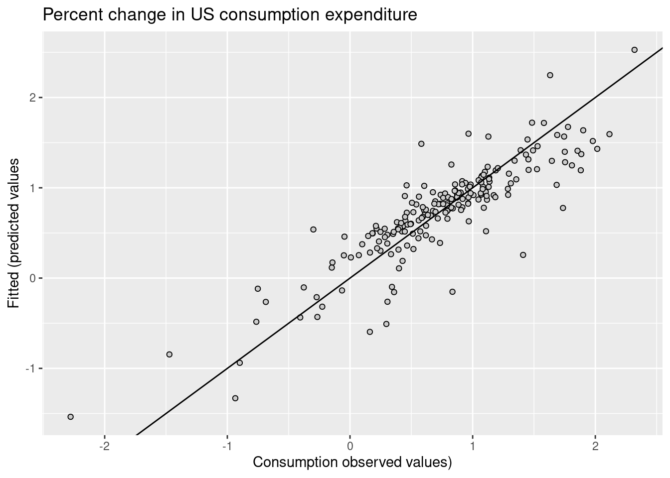

To summarise how well a linear regression model fits the data is via \(R^2\) the coefficient of determination.

The square of the correlation between the observed \(y\) values and the predicted \(\hat{y}\) values, ranges between 0 and 1.

\[R^2=\frac{\sum{(\hat{y_t}-\bar{y})^2}}{\sum{(y_t-\bar{y})^2}}\]

Residual standard error measure of how well the model has fitted the data.

\[\hat{\sigma}_e=\sqrt{\frac{1}{T-k-1}\sum_{t=1}^T{e_t^2}}\] \(k\) is the number of predictors

us_change |>
  left_join(residuals(fit_consMR), by = "Quarter") |>
  pivot_longer(Income:Unemployment,
               names_to = "regressor", values_to = "x") |>
  ggplot(aes(x = x, y = .resid)) +
  geom_point() +
  facet_wrap(. ~ regressor, scales = "free_x") +
  labs(y = "Residuals", x = "")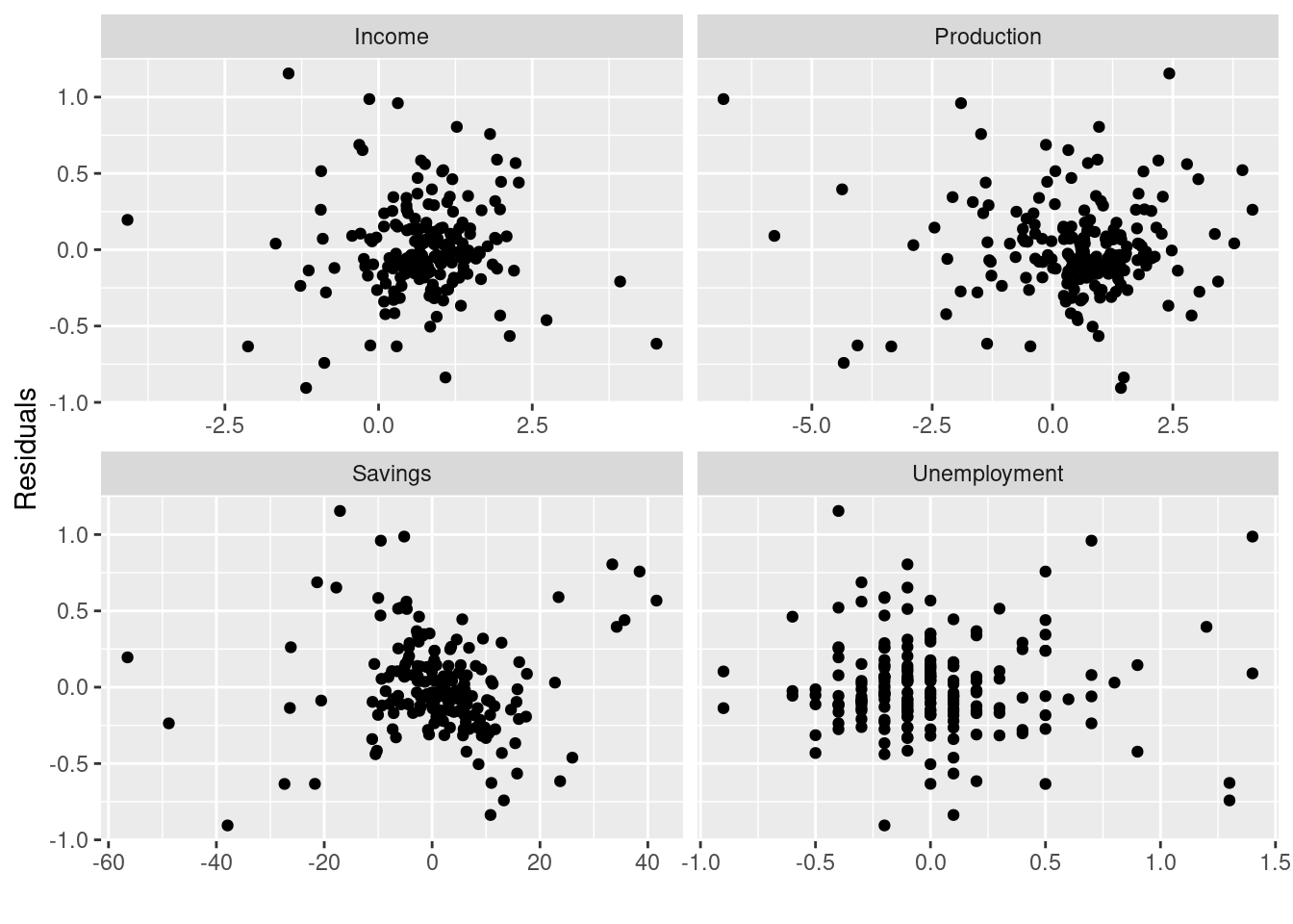

augment(fit_consMR) |>
  ggplot(aes(x = .fitted, y = .resid)) +
  geom_point() + labs(x = "Fitted", y = "Residuals")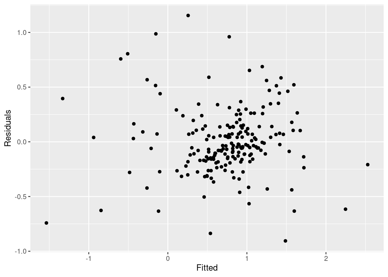

7.4.1 Example

recent_production <- aus_production |>
  filter(year(Quarter) >= 1992)


fit_beer <- recent_production |>
  model(TSLM(Beer ~ trend() + season()))

augment(fit_beer) |>
  ggplot(aes(x = Quarter)) +
  geom_line(aes(y = Beer, colour = "Data")) +
  geom_line(aes(y = .fitted, colour = "Fitted")) +
  scale_colour_manual(
    values = c(Data = "black", Fitted = "#D55E00")
  ) +
  labs(y = "Megalitres",
       title = "Australian quarterly beer production") +
  guides(colour = guide_legend(title = "Series"))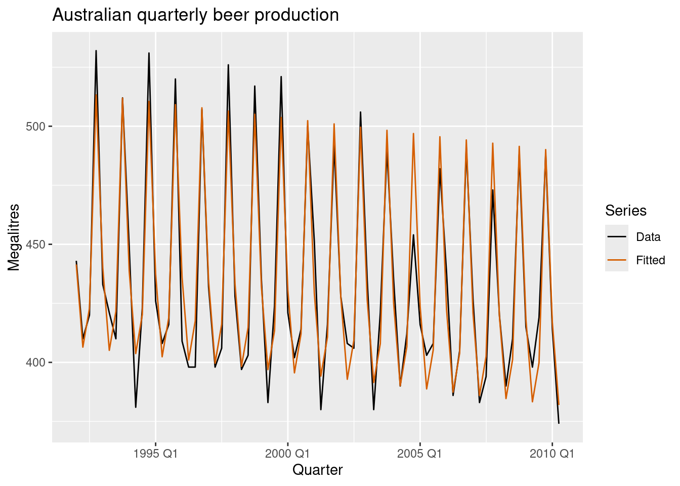

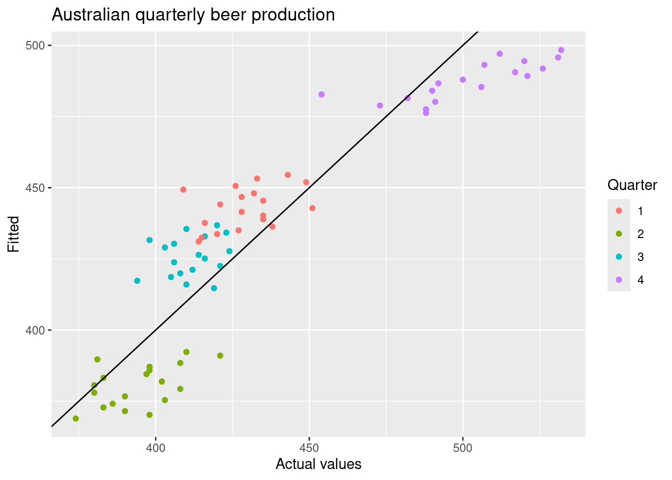
augment(fit_beer) |>
  ggplot(aes(x = Beer, y = .fitted,
             colour = factor(quarter(Quarter)))) +
  geom_point() +
  labs(y = "Fitted", x = "Actual values",
       title = "Australian quarterly beer production") +
  geom_abline(intercept = 0, slope = 1) +
  guides(colour = guide_legend(title = "Quarter"))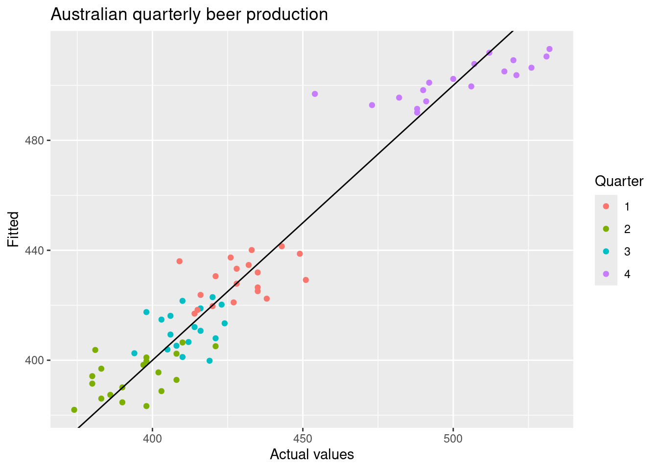

7.4.1.1 With transformation

fourier()

The maximum allowed is \(K=m/2\) where \(m\) is the seasonal period.

fourier_beer <- recent_production |>
  model(TSLM(Beer ~ trend() + fourier(K = 1)))

augment(fourier_beer) |>
  ggplot(aes(x = Quarter)) +
  geom_line(aes(y = Beer, colour = "Data")) +
  geom_line(aes(y = .fitted, colour = "Fitted")) +
  scale_colour_manual(
    values = c(Data = "black", Fitted = "#D55E00")
  ) +
  labs(y = "Megalitres",
       title = "Australian quarterly beer production") +
  guides(colour = guide_legend(title = "Series"))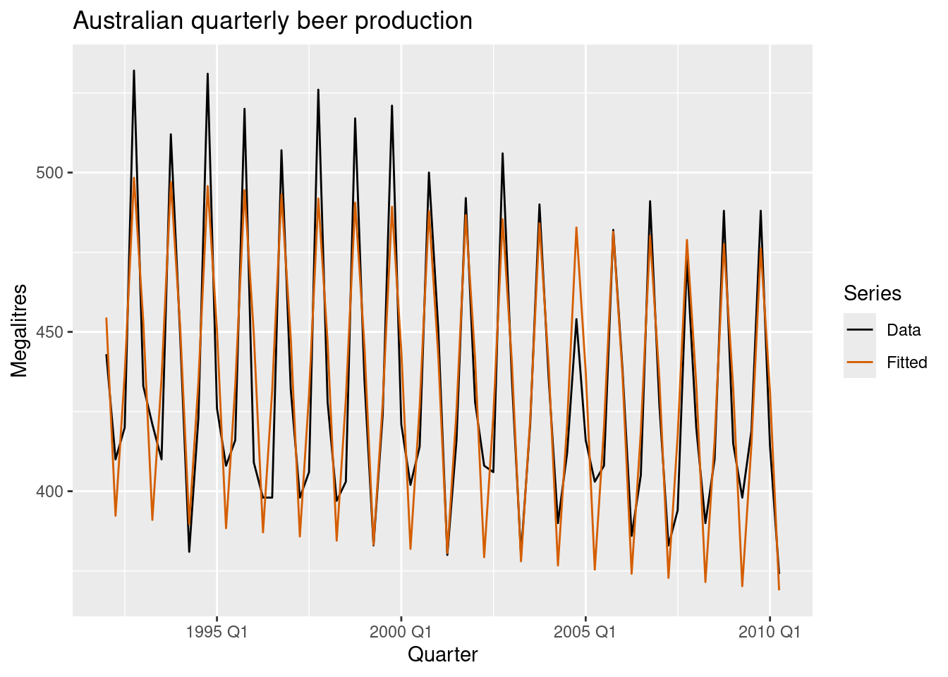

augment(fourier_beer) |>
  ggplot(aes(x = Beer, y = .fitted,
             colour = factor(quarter(Quarter)))) +
  geom_point() +
  labs(y = "Fitted", x = "Actual values",
       title = "Australian quarterly beer production") +
  geom_abline(intercept = 0, slope = 1) +
  guides(colour = guide_legend(title = "Quarter"))