PCA example

Borrowed from Introduction to Statistical Learning, USArrests is a dataset that is part of base R. The dataset is for crime statistics for the 50 US states in 1973. It contains arrests per 100,000 for three categories of crime and also the percentage of urban population.

states <- row.names(USArrests)
apply(USArrests,2, mean)

##   Murder  Assault UrbanPop     Rape 
##    7.788  170.760   65.540   21.232

cov(USArrests)

##              Murder   Assault   UrbanPop      Rape
## Murder    18.970465  291.0624   4.386204  22.99141
## Assault  291.062367 6945.1657 312.275102 519.26906
## UrbanPop   4.386204  312.2751 209.518776  55.76808
## Rape      22.991412  519.2691  55.768082  87.72916

The scale of these these is quite different, so lets center and scale the data:

USArrests_cs <- scale(USArrests)
USArrests_cov <- cov(USArrests_cs)

According to the prescription, we should find the eigensystem:

es <- eigen(USArrests_cov)
es$values

## [1] 2.4802416 0.9897652 0.3565632 0.1734301

The largest eigenvalue (and hence first principle component) corresponds to the eigenvector:

es$vectors[,1]

## [1] -0.5358995 -0.5831836 -0.2781909 -0.5434321

verify its an eigenvector:

USArrests_cov %*% es$vectors[,1]/es$values[[1]]

##                [,1]
## Murder   -0.5358995
## Assault  -0.5831836
## UrbanPop -0.2781909
## Rape     -0.5434321

Compare this to the prcomp method:

pr <- prcomp(USArrests, scale = TRUE)
pr$rotation

##                 PC1        PC2        PC3         PC4
## Murder   -0.5358995 -0.4181809  0.3412327  0.64922780
## Assault  -0.5831836 -0.1879856  0.2681484 -0.74340748
## UrbanPop -0.2781909  0.8728062  0.3780158  0.13387773
## Rape     -0.5434321  0.1673186 -0.8177779  0.08902432

es$vectors

##            [,1]       [,2]       [,3]        [,4]
## [1,] -0.5358995  0.4181809 -0.3412327  0.64922780
## [2,] -0.5831836  0.1879856 -0.2681484 -0.74340748
## [3,] -0.2781909 -0.8728062 -0.3780158  0.13387773
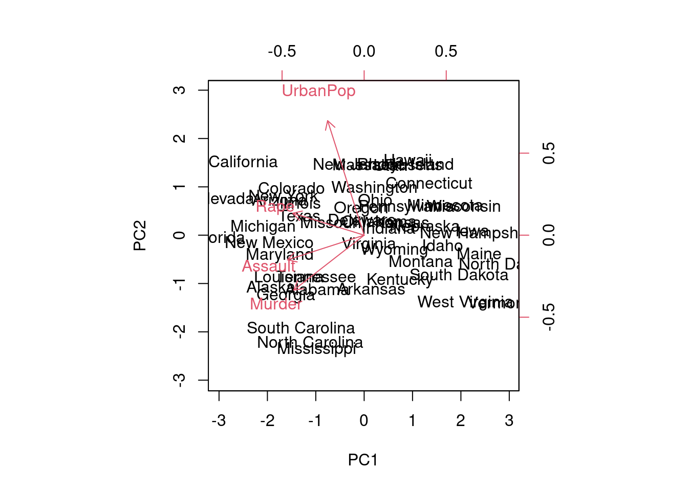
## [4,] -0.5434321 -0.1673186  0.8177779  0.08902432

We could press on and compute the data coefficients manually, but in the interest of time, we can just use biplot on the output from prcomp

biplot(pr, scale = 0)