10.3 Were Ichiro and Mike Trout unusually streaky?
One good measure of streakiness or clumpiness in the sequence is the sum of squares of the gaps between successive hits - ABDWR
To illustrate this method, consider a hypothetical player who bats 13 times with the outcomes …If the player sequence of hit/out outcomes is truly random, then all possible arrangements of the sequence of 6 hits and 7 outs are equally likely. We randomly arrange the sequence 0, 1, 0, 0, 1, 1, 0, 0, 0, 0, 1, 1, 1, find the gaps, and compute the streakiness measure. This randomization procedure is repeated many times (e.g. 1000 times)
ichiro_S <- ichiro_AB |>
  dplyr::pull(H) |>
  streaks() |>
  dplyr::filter(values == 0) |>
  dplyr::summarize(C = sum(lengths ^ 2)) |>
  dplyr::pull()
ichiro_S
## [1] 1532random_mix <- function(y) {
y |>
sample() |>
streaks() |>
dplyr::filter(values == 0) |>
dplyr::summarize(C = sum(lengths ^ 2)) |>
dplyr::pull()
}Ichiro’s line is on the right side suggesting streakiness
ggplot2::ggplot(tibble::enframe(ichiro_random), ggplot2::aes(ichiro_random)) +
  ggplot2::geom_histogram(
    ggplot2::aes(y = ggplot2::after_stat(density)), bins = 20,
    color = "blue", fill = "white"
  ) +
  ggplot2::geom_vline(xintercept = ichiro_S, linewidth = 2) +
  ggplot2::annotate(
    geom = "text", x = ichiro_S * 1.15,
    y = 0.0010, label = "OBSERVED", size = 5
) 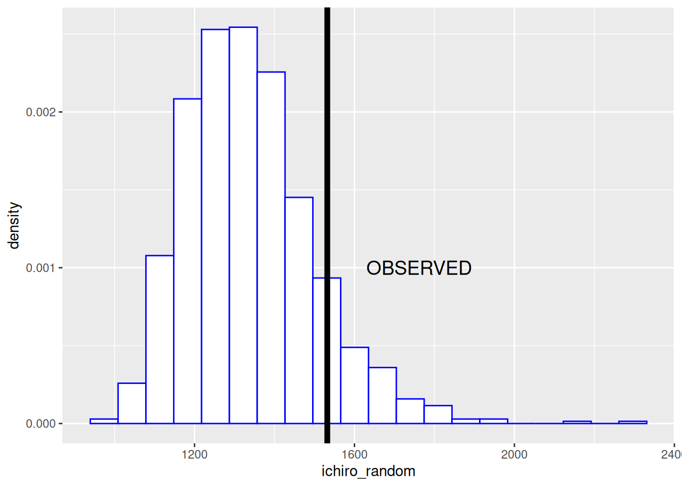
##     0%    10%    20%    30%    40%    50%    60%    70%    80%    90%   100%
##  998.0 1153.8 1202.0 1242.0 1282.0 1322.0 1360.0 1404.0 1460.0 1536.2 2320.0
Create a function for a given playerid
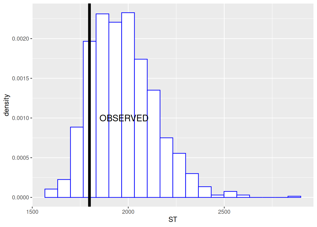
clump_test <- function(data, playerid) {
  player_ab <- data |>
    dplyr::filter(bat_id == playerid, ab_fl == TRUE) |>
    dplyr::mutate(
      H = ifelse(h_fl > 0, 1, 0),
      date = substr(game_id, 4, 12)
    ) |>
    dplyr::arrange(date)

  stat <- player_ab |>
    dplyr::pull(H) |>
    streaks() |>
    dplyr::filter(values == 0) |>
    dplyr::summarize(C = sum(lengths ^ 2)) |>
    dplyr::pull()

  ST <- 1:1000 |>
    purrr::map_int(~random_mix(player_ab$H))

  ggplot2::ggplot(tibble::enframe(ST), ggplot2::aes(ST)) +
    ggplot2::geom_histogram(
      ggplot2::aes(y = ggplot2::after_stat(density)), bins = 20,
      color = "blue", fill = "white"
    ) +
    ggplot2::geom_vline(xintercept = stat, linewidth = 2) +
    ggplot2::annotate(
      geom = "text", x = stat * 1.10,
      y = 0.0010, label = "OBSERVED", size = 5
    )
}
Is Mike Trout considered streaky in 2016?