11.13 Exercises

11.13.1 1. Runs Scored at the Astrodome

# dbSendQuery(con, "TRUNCATE TABLE gamelogs;")
# map(1965:1999, append_game_logs, conn = con)
# 
# query <- '
# SELECT
#     SUBSTRING("Date"::text FROM 1 FOR 4) AS year,
#     COUNT(*) AS num_games
# FROM
#     gamelogs
# GROUP BY
#     year
# ORDER BY
#     year;
# '
# 
# dbGetQuery(con, query)

Select games featuring the Astros (as either the home or visiting team) during the years when the Astrodome was their home park (i.e., from 1965 to 1999) using dplyr to get SQL query.

# gamelogs |> 
#      select(Date, ParkID, HomeTeam, VisitingTeam, HomeRunsScore, VisitorRunsScored) |> 
#      filter(HomeTeam == 'HOU' | VisitingTeam == 'HOU') |> 
#      show_query()
# 
# query <- '
# SELECT
#   "Date",
#   "ParkID",
#   "HomeTeam",
#   "VisitingTeam",
#   "HomeRunsScore",
#   "VisitorRunsScored"
# FROM "gamelogs"
# WHERE ("HomeTeam" = \'HOU\' OR "VisitingTeam" = \'HOU\');
# '

# astros <- dbGetQuery(con, query) |> 
#      mutate(
#           total_runs_scored = HomeRunsScore + VisitorRunsScored, 
#           astrodome = ParkID == "HOU02"
#           )
astros <- read_rds('./data/astros.rds')

head(astros, 10)

##        Date ParkID HomeTeam VisitingTeam HomeRunsScore VisitorRunsScored
## 1  19650412  HOU02      HOU          PHI             0                 2
## 2  19650414  NYC17      NYN          HOU             6                 7
## 3  19650415  NYC17      NYN          HOU             5                 4
## 4  19650417  PIT06      PIT          HOU             3                 2
## 5  19650418  PIT06      PIT          HOU             1                 3
## 6  19650418  PIT06      PIT          HOU             5                 4
## 7  19650419  PHI11      PHI          HOU             8                 0
## 8  19650420  PHI11      PHI          HOU             2                 1
## 9  19650421  PHI11      PHI          HOU             4                11
## 10 19650423  HOU02      HOU          PIT             4                 3
##    total_runs_scored astrodome
## 1                  2      TRUE
## 2                 13     FALSE
## 3                  9     FALSE
## 4                  5     FALSE
## 5                  4     FALSE
## 6                  9     FALSE
## 7                  8     FALSE
## 8                  3     FALSE
## 9                 15     FALSE
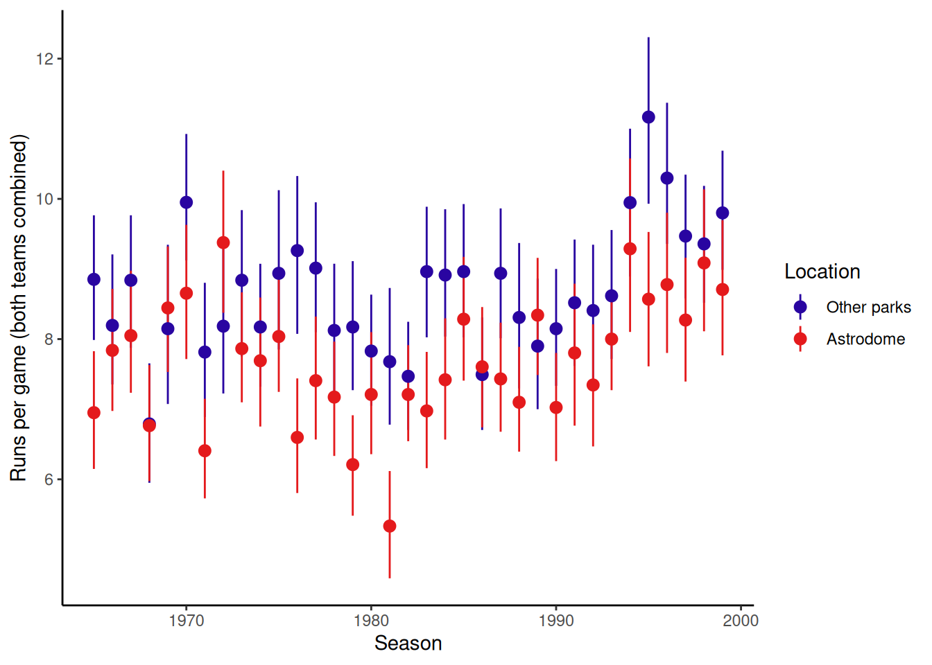
## 10                 7      TRUE

11.13.2 2. Draw a plot to visually compare through the years the runs scored (both teams combined) in games played at the Astrodome and in other ballparks.

astros |> 
     select(Date, total_runs_scored, astrodome) |> 
     
     ggplot(aes(x = year(ymd(Date)), y = total_runs_scored, color = astrodome)) + 
     stat_summary(fun.data = "mean_cl_boot") + 
     xlab("Season") +
     ylab("Runs per game (both teams combined)") +
     scale_color_manual(
          name = "Location", values = crc_fc,
          labels = c("Other parks", "Astrodome")
     )

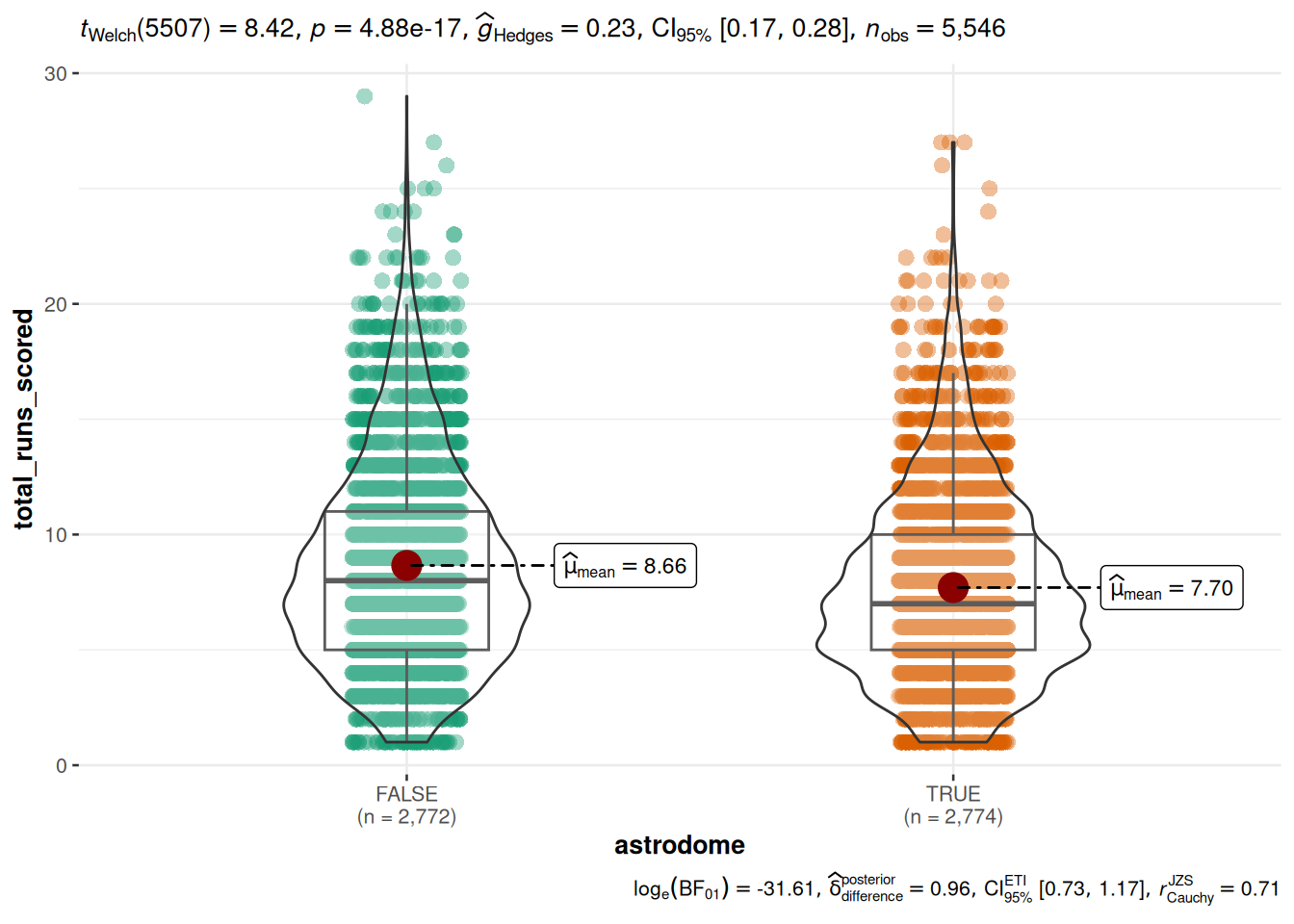
Another visualization (ggbetweenstats)

set.seed(1234)
astros |> 
     ggbetweenstats(
          x = astrodome, 
          y = total_runs_scored
     )

astros |> 
     group_by(year(ymd(Date)), astrodome) |> 
     summarise(
          avg_runs = mean(total_runs_scored), .groups = 'drop'
          ) |> 
     rename(date = 1) |> 
     pivot_wider(
          id_cols = 'date', 
          names_from = 'astrodome', 
          values_from = 'avg_runs'
     ) |> 
     rename('Other_parks' = 2, Astrodome = 3) |> 
     mutate(delta = Other_parks - Astrodome) |> 
     
     ggplot(aes(x = date, y = delta)) + 
     geom_point(size = 2, color = 'steelblue') + 
     geom_hline(yintercept=0, linetype="dashed", color = "red")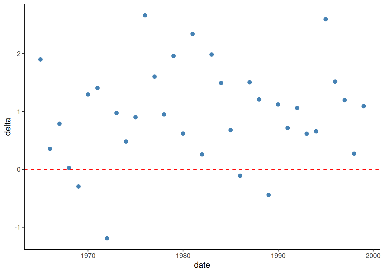

Disconnect db connection

# dbDisconnect(conn = con)