11.9 Coors Field and run scoring

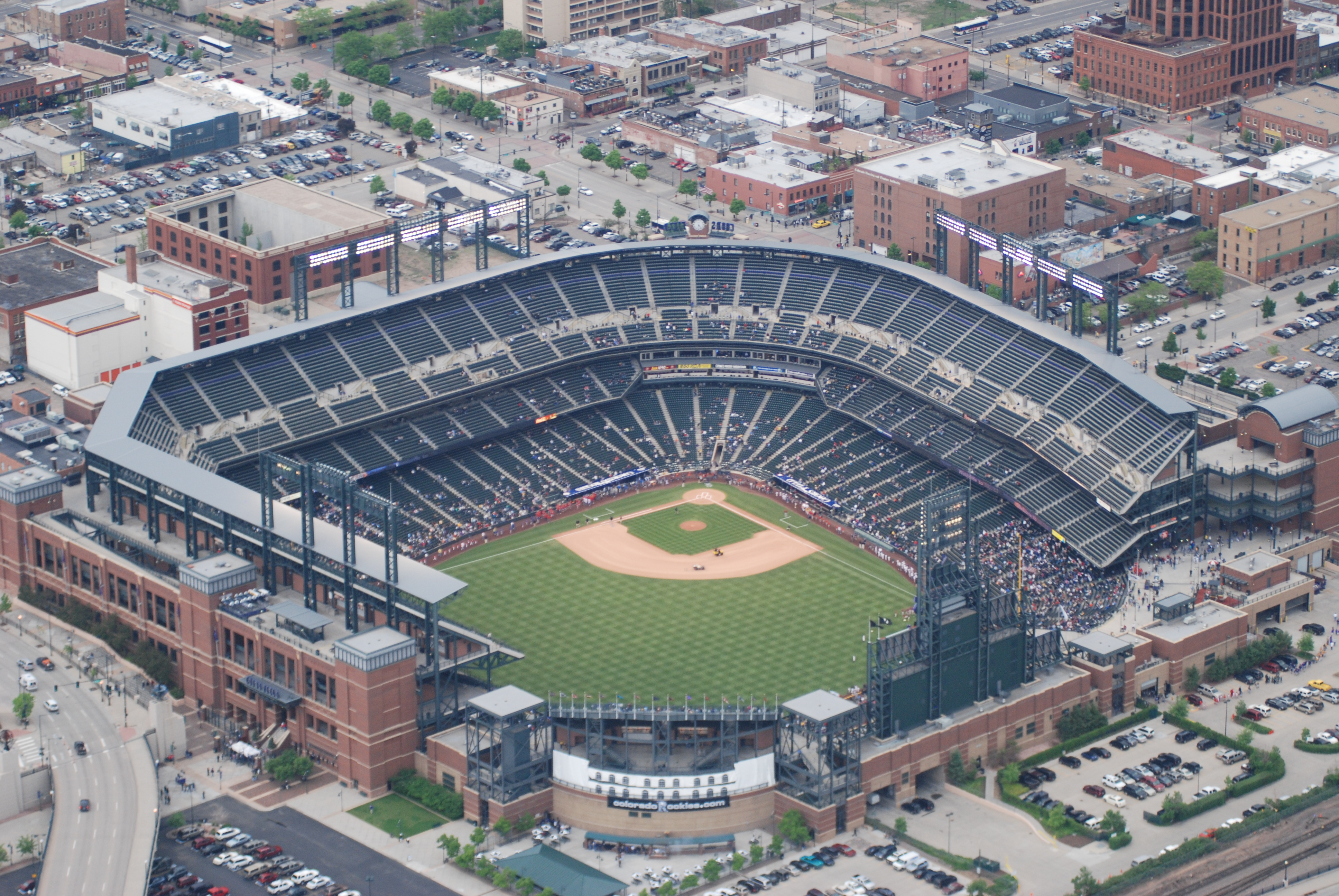
Coors Field Aerial View

Batting Park Factors (BPF)

“is a baseball statistic that indicates the difference between runs scored in a team’s home and road games” - Wikipedia

The formula most common used is:

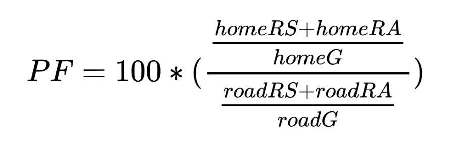
BPF formula

Look at the games played by the Rockies—either at home or on the road—since 1995.

# query <- '
# SELECT "Date", "ParkID", "VisitingTeam", "HomeTeam", 
#   "VisitorRunsScored" AS awR, "HomeRunsScore" AS hmR
# FROM "gamelogs"
# WHERE ("HomeTeam" = \'COL\') OR ("VisitingTeam" = \'COL\') 
#   AND "Date" > 19950000;
# '
# 
# rockies_games <- dbGetQuery(con, query)

rockies_games <- gamelogs |> 
  select(Date, ParkID, VisitingTeam, HomeTeam, 
         awR = VisitorRunsScored, 
         hmR = HomeRunsScore) |> 
  filter(HomeTeam == 'COL' | VisitingTeam == 'COL', 
         Date > 19950000)

head(rockies_games, 10)

## # A tibble: 10 × 6
##        Date ParkID VisitingTeam HomeTeam   awR   hmR
##       <dbl> <chr>  <chr>        <chr>    <dbl> <dbl>
##  1 19950426 DEN02  NYN          COL          9    11
##  2 19950427 DEN02  NYN          COL          7     8
##  3 19950428 HOU02  COL          HOU          2     1
##  4 19950429 HOU02  COL          HOU          2     1
##  5 19950430 HOU02  COL          HOU          1     3
##  6 19950501 DEN02  SDN          COL          3     8
##  7 19950502 DEN02  SDN          COL          5     6
##  8 19950503 DEN02  SDN          COL          7    12
##  9 19950505 DEN02  LAN          COL          6     4
## 10 19950506 DEN02  LAN          COL         17    11

Compute the sum of runs scored in each game by adding the runs scored by the home team and the visiting team. We also add a new column coors indicating whether the game was played at Coors Field.

rockies_games <- rockies_games |>
     mutate(
          runs = awR + hmR, 
          coors = ParkID == "DEN02"
     )

head(rockies_games, 10)

## # A tibble: 10 × 8
##        Date ParkID VisitingTeam HomeTeam   awR   hmR  runs coors
##       <dbl> <chr>  <chr>        <chr>    <dbl> <dbl> <dbl> <lgl>
##  1 19950426 DEN02  NYN          COL          9    11    20 TRUE 
##  2 19950427 DEN02  NYN          COL          7     8    15 TRUE 
##  3 19950428 HOU02  COL          HOU          2     1     3 FALSE
##  4 19950429 HOU02  COL          HOU          2     1     3 FALSE
##  5 19950430 HOU02  COL          HOU          1     3     4 FALSE
##  6 19950501 DEN02  SDN          COL          3     8    11 TRUE 
##  7 19950502 DEN02  SDN          COL          5     6    11 TRUE 
##  8 19950503 DEN02  SDN          COL          7    12    19 TRUE 
##  9 19950505 DEN02  LAN          COL          6     4    10 TRUE 
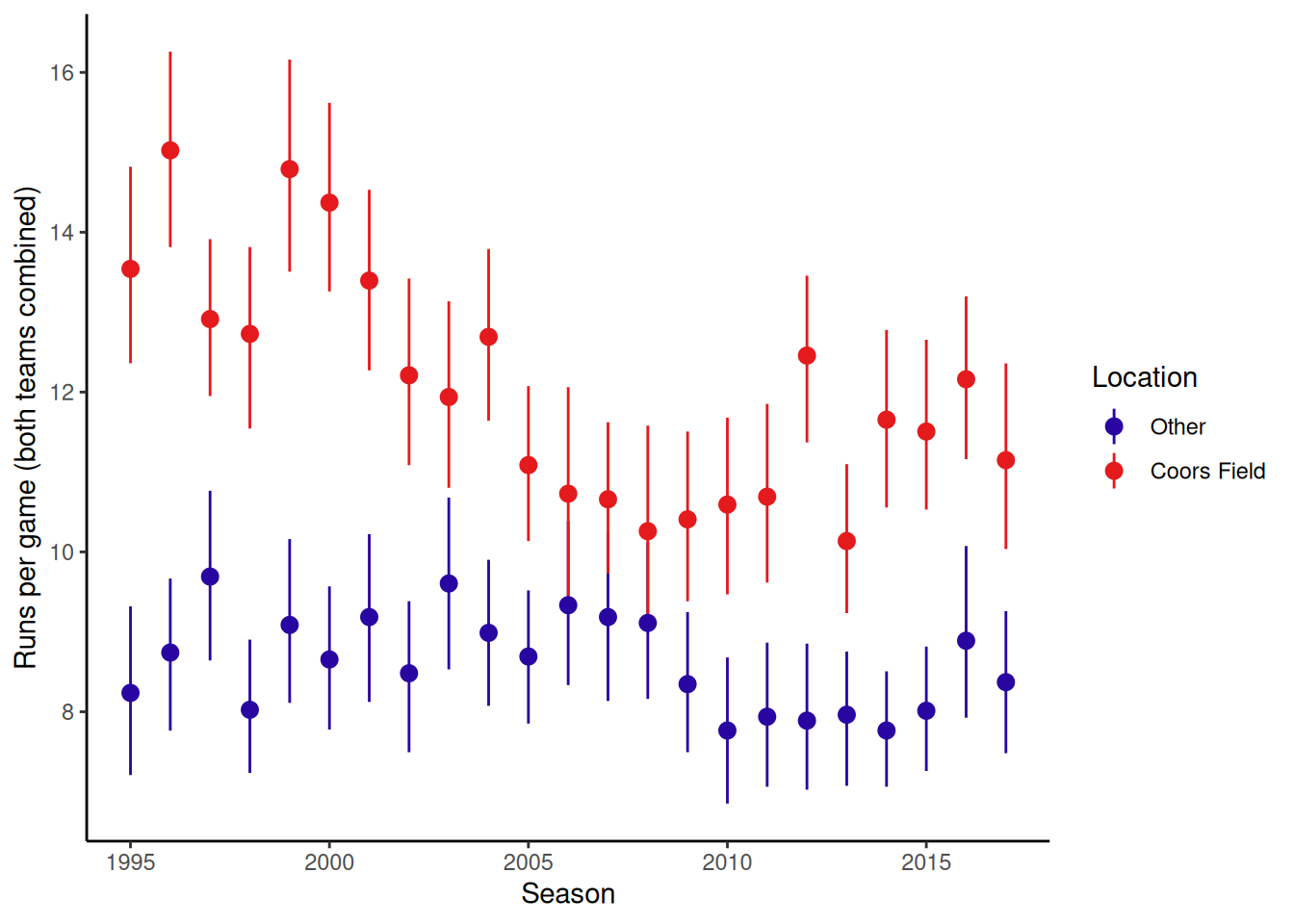
## 10 19950506 DEN02  LAN          COL         17    11    28 TRUE

Now, let’s compare the offensive output by the Rockies and their opponents at Coors and other ballparks.

rockies_games |> 
     ggplot(aes(x = year(ymd(Date)), y = runs, color = coors)) +
     stat_summary(fun.data = "mean_cl_boot") + 
     xlab("Season") +
     ylab("Runs per game (both teams combined)") +
     scale_color_manual(
          name = "Location", values = crc_fc,
          labels = c("Other", "Coors Field")
     )

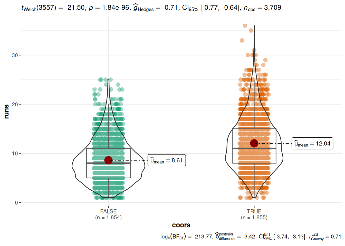
Another approach using ggbetweenstats() from the ggstatsplot package.

set.seed(1234)
rockies_games |> 
     ggbetweenstats(
          x = coors, 
          y = runs
     )