11.11 Home run park factor
Explore the stadium effect on home runs in 1996.
##   away_team_id home_team_id event_cd was_hr
## 1          SFN          ATL        2      0
## 2          SFN          ATL        2      0
## 3          SFN          ATL       18      0
## 4          SFN          ATL        2      0
## 5          SFN          ATL       23      1
## 6          SFN          ATL        2      0
Compute the frequency of home runs per batted ball for all MLB teams both at home and on the road.
ev_away <- hr_PF |>
     group_by(team_id = away_team_id) |>
     summarize(hr_event = mean(was_hr)) |>
     mutate(type = "away")

ev_home <- hr_PF |>
     group_by(team_id = home_team_id) |>
     summarize(hr_event = mean(was_hr)) |>
     mutate(type = "home")
Combine the two resulting data frames and use the pivot_wider() function to put the home and away home run frequencies side-by-side.
ev_compare <- ev_away |>
     bind_rows(ev_home) |>
     pivot_wider(names_from = type, values_from = hr_event)

ev_compare |>
  head(10)
## # A tibble: 10 × 3
## team_id away home
## <chr> <dbl> <dbl>
## 1 ATL 0.0323 0.0372
## 2 BAL 0.0488 0.0477
## 3 BOS 0.0385 0.0443
## 4 CAL 0.0387 0.0483
## 5 CHA 0.0424 0.0349
## 6 CHN 0.0374 0.0407
## 7 CIN 0.0403 0.0393
## 8 CLE 0.0440 0.0372
## 9 COL 0.0341 0.0538
## 10 DET 0.0457 0.0506Compute the 1996 home run park factors with the the following code, and use arrange() to display the ballparks with the largest and smallest park factors.
ev_compare <- ev_compare |>
     mutate(pf = 100 * home / away)

ev_compare |>
     arrange(desc(pf)) |>
     slice_head(n = 6)
## # A tibble: 6 × 4
## team_id away home pf
## <chr> <dbl> <dbl> <dbl>
## 1 COL 0.0341 0.0538 158.
## 2 CAL 0.0387 0.0483 125.
## 3 ATL 0.0323 0.0372 115.
## 4 BOS 0.0385 0.0443 115.
## 5 DET 0.0457 0.0506 111.
## 6 SDN 0.0294 0.0320 109.Coors Field is at the top of the HR-friendly list, displaying an extreme value of 158—this park boosted home run frequency by over 50% in 1996!
## # A tibble: 6 × 4
##   team_id   away   home    pf
##   <chr>    <dbl>  <dbl> <dbl>
## 1 LAN     0.0360 0.0256  71.2
## 2 HOU     0.0344 0.0272  79.1
## 3 NYN     0.0363 0.0289  79.5
## 4 CHA     0.0424 0.0349  82.2
## 5 CLE     0.0440 0.0372  84.6
## 6 FLO     0.0316 0.0271  85.7
Dodger Stadium in Los Angeles, featuring a home run park factor of 71, meaning that it suppressed home runs by nearly 30% relative to the league average park.
# lollipop chart
ev_compare |>
     arrange(pf) |>
     mutate(
          pf_flag = ifelse(pf > 100, TRUE, FALSE)
     ) |>

     ggplot(aes(x = pf, y = reorder(team_id, pf), color = pf_flag)) +
     geom_segment(aes(x = 100, y = team_id, xend = pf, yend = team_id)) +
     geom_point() +
     scale_color_manual(values = c(crc_fc[2], crc_fc[1])) +
     labs(
          x = 'Home Run Park Factor',
          y = NULL,
          title = '1996 Seaons Home Run Park Factor by Team'
     ) +
     theme_classic() +
     theme(legend.position = "none")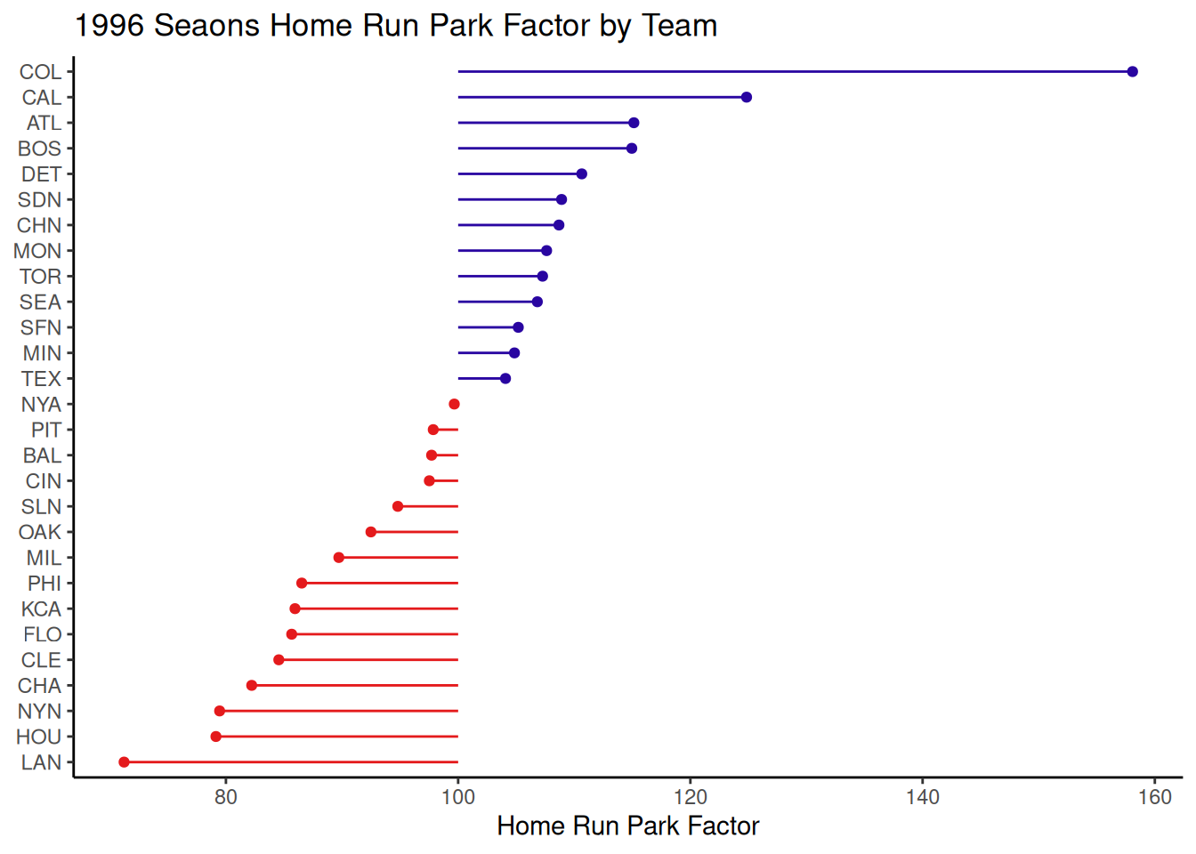
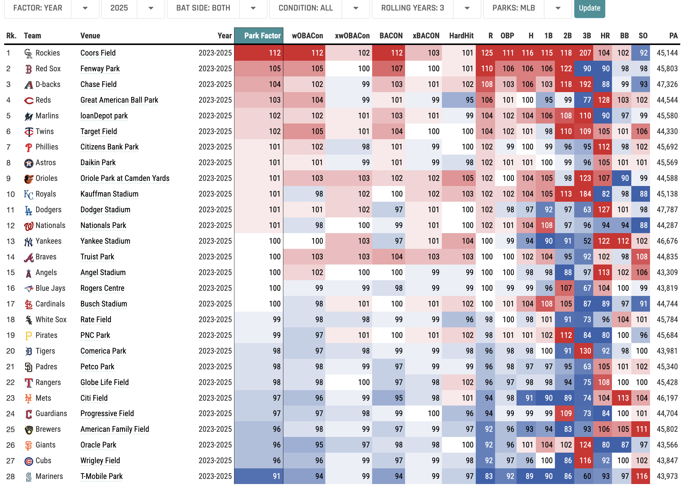
How has the PF (Park Factors) rating change since?