11.7 Querying Data from R

Let’s compare the attendance of two Chicago teams by day of the week since the 2006 season. - CHA - Chicago White Sox - CHN - Chicago Cubs

# query <- '
# SELECT "Date", "HomeTeam", "DayOfWeek", "Attendance"
# FROM "gamelogs"
# WHERE ("Date" > 20060101.0) 
#      AND ("HomeTeam" IN (\'CHN\', \'CHA\'))
# '
# 
# chi_attendance <- dbGetQuery(con, query) 
# slice_head(chi_attendance, n = 6)

# using dplyr (tidyverse)
chi_attendance <- gamelogs |>
     filter(Date > 20060101, HomeTeam %in% c('CHN', 'CHA')) |>
     select(Date, HomeTeam, DayOfWeek, Attendance)

chi_attendance |> 
  head()

## # A tibble: 6 × 4
##       Date HomeTeam DayOfWeek Attendance
##      <dbl> <chr>    <chr>          <dbl>
## 1 20060402 CHA      Sun            38802
## 2 20060404 CHA      Tue            37591
## 3 20060405 CHA      Wed            33586
## 4 20060407 CHN      Fri            40869
## 5 20060408 CHN      Sat            40182
## 6 20060409 CHN      Sun            39839

# show_query()
# gamelogs |>
#      filter(Date > 20060101, HomeTeam %in% c('CHN', 'CHA')) |>
#      select(Date, HomeTeam, DayOfWeek, Attendance) |>
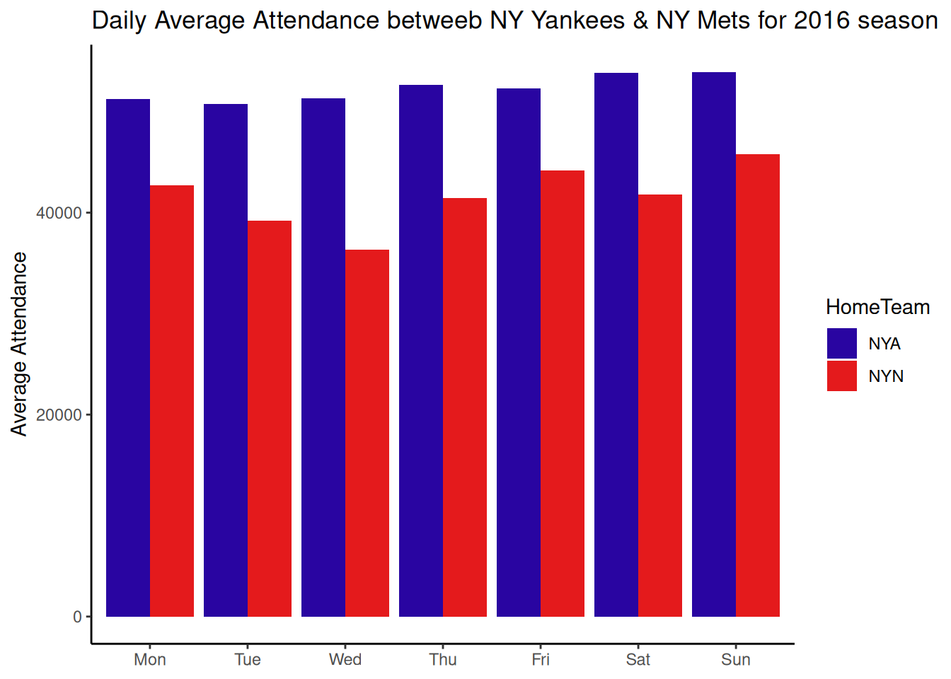
#      show_query()

Another exercise: let’s compare for New York Yankees and Mets daily average attendance.

gamelogs |>
     filter(Date >= 20060101, Date <= 20061101, HomeTeam %in% c('NYN', 'NYA')) |>
     select(Date, HomeTeam, DayOfWeek, Attendance) |> 
     group_by(HomeTeam, DayOfWeek) |> 
     summarise(average_attendance = mean(Attendance, na.rm = TRUE), 
               .groups = 'drop') |> 
     as_tibble() |> 

     mutate(dayofweek = DayOfWeek %>% 
                 factor(levels = c('Mon', 'Tue', 'Wed', 'Thu', 'Fri', 'Sat', 'Sun'), 
                        ordered = TRUE)) |> 
     arrange(HomeTeam, dayofweek) |> 
     
     # plot attendance by team
     ggplot(aes(x = dayofweek, y = average_attendance, fill = HomeTeam)) + 
     geom_col(position = 'dodge') + 
     scale_fill_manual(values = c(crc_fc[1], crc_fc[2])) + 
     labs(
       x = NULL, 
       y = 'Average Attendance', 
       title = 'Daily Average Attendance betweeb NY Yankees & NY Mets for 2016 season'
         ) + 
    theme_classic()