The Great Streak

• play-by-play now available on Retrosheet and downloadable via baseballr package
• we gather our data from Baseball Reference and book’s package

library(abdwr3edata)
joe <- dimaggio_1941

# Check DiMaggio's batting average for the season
joe |> dplyr::summarize(AVG = sum(H) / sum(AB))

## # A tibble: 1 × 1
##     AVG
##   <dbl>
## 1 0.357

A hitting streak is commonly defined as the number of consecutive games in which a player gets at least one base hit. - Analyzing Baseball Data with R

However…

A consecutive hitting streak shall not be terminated if a batter’s plate appearance results in a base on balls, hit batsman, defensive interference or obstruction or a sacrifice bunt. A sacrifice fly shall terminate the streak - MLB Official Rulebook

joe <- joe |> 
  dplyr::mutate(had_hit = dplyr::if_else(H > 0, 1, 0))

dplyr::pull(joe, had_hit)

##   [1] 1 1 1 1 1 1 1 1 0 0 0 1 1 1 0 1 1 0 0 1 0 0 0 1 1 1 0 0 1 1 1 1 1 1 1 1 1
##  [38] 1 1 1 1 1 1 1 1 1 1 1 1 1 1 1 1 1 1 1 1 1 1 1 1 1 1 1 1 1 1 1 1 1 1 1 1 1
##  [75] 1 1 1 1 1 1 1 1 1 1 0 1 1 1 1 1 1 1 1 1 1 1 1 1 1 1 1 0 0 1 1 1 1 0 0 1 1
## [112] 0 0 0 1 1 1 1 0 0 0 1 1 1 1 1 1 1 0 1 0 1 1 1 1 1 0 1 1

What if we wanted to calculate all the hitting streaks for a particular player?

streaks <- function(y) {
  x <- rle(y)
  class(x) <- "list"
  tibble::as_tibble(x)
}

joe |> 
  dplyr::pull(had_hit) |> 
  streaks() |>
  dplyr::filter(values == 1) |>
  dplyr::pull(lengths)

##  [1]  8  3  2  1  3 56 16  4  2  4  7  1  5  2

We can also find streaks of no hits. DiMaggio’s longest in 1941 was only 3 games

joe |> 
  dplyr::pull(had_hit) |> 
  streaks() |>
  dplyr::filter(values == 0) |>
  dplyr::pull(lengths)

##  [1] 3 1 2 3 2 1 2 2 3 3 1 1 1

10.0.1 Moving Batting Averages

• Suppose we are interested in a player’s batting average over a moving window (e.g. a stretch of 10 games 1-10, 2-11, 3-12…)
• We create a new function moving_average featuring rollmean() and rollsum() from the zoo package

# transmute is superseded because you can perform the same job with mutate(.keep = "none").

library(zoo)

## 
## Attaching package: 'zoo'

## The following objects are masked from 'package:base':
## 
##     as.Date, as.Date.numeric

moving_average <- function(df, width) {
  N <- nrow(df)
  df |>
    dplyr::transmute(
      Game = zoo::rollmean(1:N, k = width, fill = NA), 
      Average = zoo::rollsum(H, width, fill = NA) /
        rollsum(AB, width, fill = NA)
    )
}

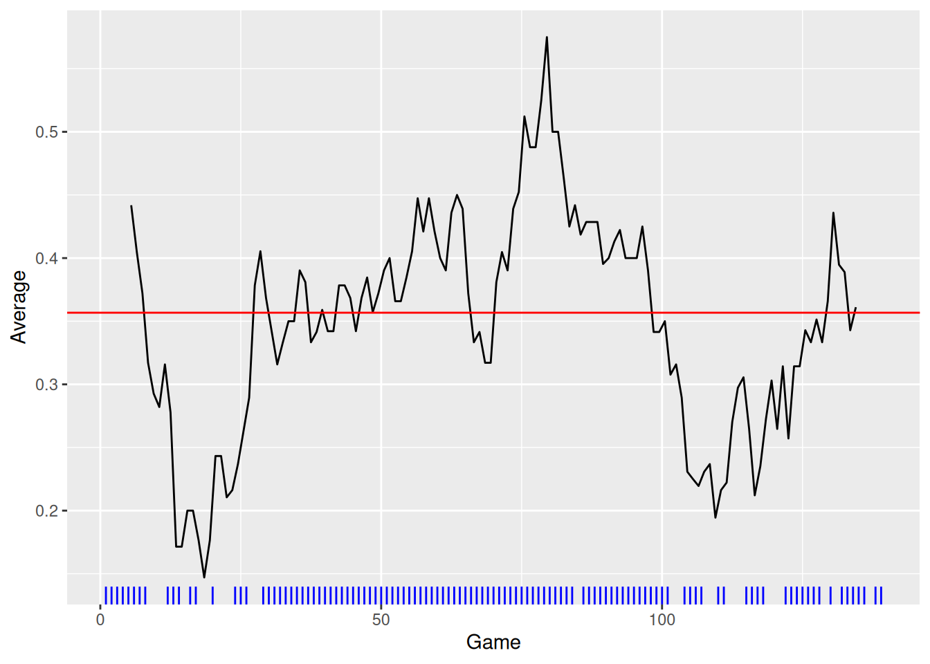
We then calculate a moving average for a 10 game window for Joe DiMaggio and plot this along with his season average as well as games where he recorded a hit.

joe_ma <- moving_average(joe, 10)

ggplot2::ggplot(joe_ma, ggplot2::aes(Game, Average)) +
  ggplot2::geom_line() +
  ggplot2::geom_hline(
    data = dplyr::summarize(joe, bavg = sum(H)/sum(AB)), 
    ggplot2::aes(yintercept = bavg), color = "red"
  ) +
  ggplot2::geom_rug(
    data = dplyr::filter(joe, had_hit == 1),
    ggplot2::aes(Rk, .3 * had_hit), sides = "b", 
    color = "blue"
  )

## Warning: Removed 9 rows containing missing values or values outside the scale range
## (`geom_line()`).