4.7 Case Studies
4.7.1 2011 Red Sox
BOS_2011 <- retro_gl_2011 |> #Retrosheet data (via abdwr3edata)
  filter(HomeTeam == "BOS" | VisitingTeam == "BOS") |>
  select(VisitingTeam, HomeTeam, VisitorRunsScored, HomeRunsScore) |>
  mutate(ScoreDiff = ifelse(HomeTeam == "BOS",
    HomeRunsScore - VisitorRunsScored,
    VisitorRunsScored - HomeRunsScore),
    W_bool = ifelse(ScoreDiff > 0, "win", "loss"))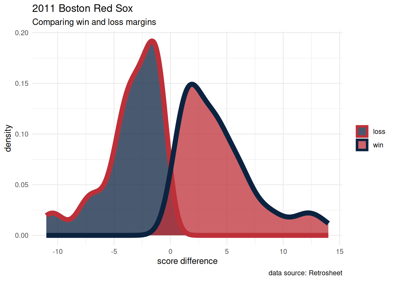
graph code
BOS_2011 |>
  ggplot(aes(x = ScoreDiff)) +
  geom_density(aes(color = W_bool,
                   fill = W_bool),
               alpha = 0.75,
               linewidth = 3) +
  labs(title = "2011 Boston Red Sox",
       subtitle = "Comparing win and loss margins",
       caption = "data source: Retrosheet",
       x = "score difference") +
  scale_color_manual(values = c("#BD3039", "#0C2340")) +
  scale_fill_manual(values = c("#0C2340", "#BD3039")) +
  theme_minimal() +
  theme(legend.position = "right",
        legend.title=element_blank())
The 2011 Red Sox had their victories decided by a larger margin than their losses (4.3 vs -3.5 runs on average), leading to their underperformance of the Pythagorean prediction
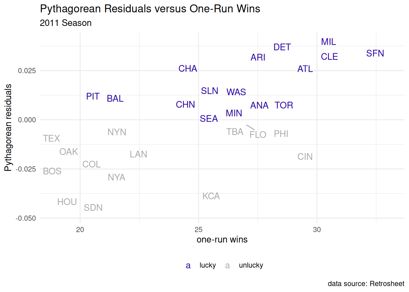
4.7.2 Clutch Performance
Here, we are tracking performance in games won with a difference of just one run.
graph code
one_run_wins <- retro_gl_2011 |>
  select(VisitingTeam, HomeTeam, VisitorRunsScored, HomeRunsScore) |>
  mutate(winner = ifelse(HomeRunsScore > VisitorRunsScored, HomeTeam, VisitingTeam),
    diff = abs(VisitorRunsScored - HomeRunsScore)
  ) |>
  filter(diff == 1) |>
  group_by(winner) |>
  summarize(one_run_w = n())

teams2011 <- ch4_data |>
  filter(yearID == 2011) |>
  mutate(teamID = if_else(teamID == "LAA", "ANA", as.character(teamID))
  ) |>
  inner_join(one_run_wins, by = c("teamID" = "winner"))

teams2011 |>
  mutate(luck = ifelse(resid_pyt > 0, "lucky", "unlucky")) |>
  ggplot(aes(x = one_run_w, y = resid_pyt)) +
  #geom_point() +
  geom_text_repel(aes(color = luck, label = teamID)) +
  xlab("One run wins") + ylab("Pythagorean residuals") +
  labs(title = "Pythagorean Residuals versus One-Run Wins",
       subtitle = "2011 Season",
       caption = "data source: Retrosheet",
       x = "one-run wins") +
  scale_color_manual(values = c("#2905A1", "#AAAAAA")) +
  theme_minimal() +
  theme(legend.position = "bottom",
        legend.title=element_blank())