9.11 Simulate Many Seasons

We can wrap the previous codes into a simulate_1968 function

simulate_1968 <- function(s_talent = 0.20){ ... }

function code

simulate_1968 <- function(s_talent = 0.20){
  teams_68 <- teams_68 |>
    mutate(talent = rnorm(10, 0, s_talent))
  
  # increase chances of Cardinals' and Tigers' success
  teams_68$talent[teams_68$teamID == "DET"] <- rnorm(1, 0.3, 0.05)
  teams_68$talent[teams_68$teamID == "SLN"] <- rnorm(1, 0.27, 0.04)
  
  schedule_talent <- schedule |>
    inner_join(teams_68, join_by(lgID, Home == teamID)) |>
    rename(talent_home = talent) |>
    inner_join(teams_68, join_by(lgID, Visitor == teamID)) |>
    rename(talent_visitor = talent)
  
  schedule_talent <- schedule_talent |> 
    mutate(
      prob_home = exp(talent_home) /
        (exp(talent_home) + exp(talent_visitor))
    )
  
  schedule_talent <- schedule_talent |>
    mutate(
      outcome = rbinom(nrow(schedule_talent), 1, prob_home),
      winner = if_else(outcome == 1, Home, Visitor)
    )
  
  results <- schedule_talent |> 
    group_by(winner) |>
    summarize(Wins = n()) |>
    inner_join(teams_68, by = c("winner" = "teamID"))
}

and use the rep function to simulate 100 copies of the 1968 season.

set.seed(20250611)
many_results <- rep(0.20, 100) |>
  map(simulate_1968) |>
  list_rbind() |>
  rename(team = winner)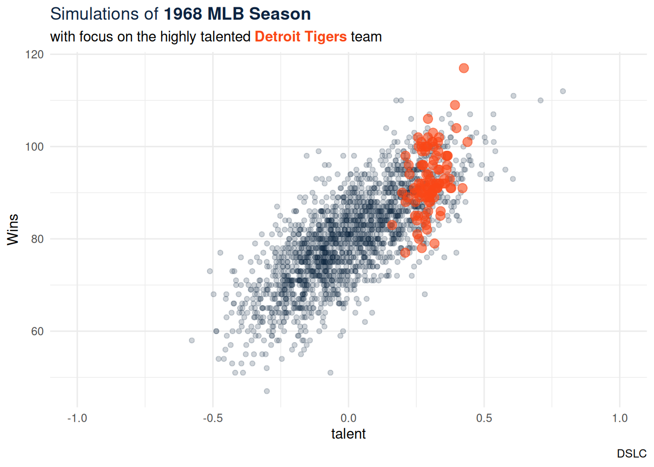

graph code

title_text <- "<span style='color:#0C2340'>Simulations of **1968 MLB Season**</span>"
subtitle_text <- "with focus on the highly talented <span style='color:#FA4616'>**Detroit Tigers**</span> team"

many_results |>
  ggplot() +
  geom_point(aes(x = talent, y = Wins),
             alpha = 0.2,
             color = "#0C2340",
             data = many_results |>
               filter(team != "DET")) +
  geom_point(aes(x = talent, y = Wins),
             alpha = 0.6,
             size = 3,
             color = "#FA4616",
             data = many_results |>
               filter(team == "DET")) +
  labs(title = title_text,
       subtitle = subtitle_text,
       caption = "DSLC") +
  theme_minimal() +
  theme(plot.subtitle = ggtext::element_markdown(),
        plot.title = ggtext::element_markdown()) +
  xlim(-1,1)

• average team \(T = 0\) tend to win about 81 games.
• positive correlation: more talent \(\Rightarrow\) more wins

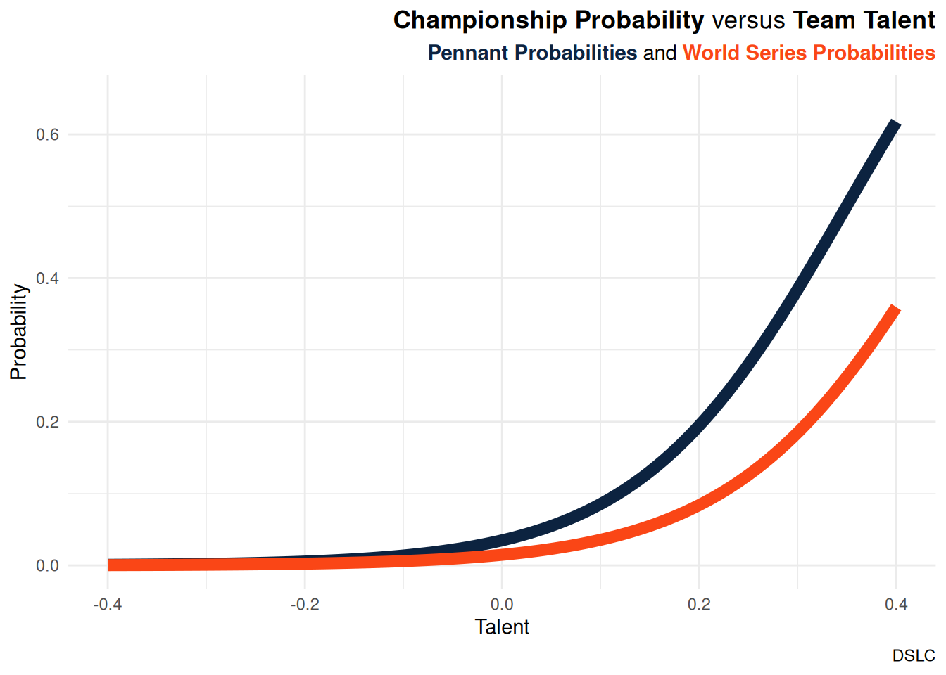
9.11.1 Parity

What is the relationship between a team’s talent and its post-season success?

set.seed(20250611)
many_results <- rep(0.20, 100) |>
  map(abdwr3edata::one_simulation_68) |>
  list_rbind()

\[P(\text{win championship}|T) = \frac{e^{a+bT}}{1 + e^{a+bT}}\]

fit1 <- glm(
  Winner.Lg ~ Talent,
  data = many_results, family = binomial
)
fit2 <- glm(
  Winner.WS ~ Talent,
  data = many_results, family = binomial
)

graph code

tdf <- tibble(
  Talent =  seq(-0.4, 0.4, length.out = 100)
)

title_text <- "**Championship Probability** versus **Team Talent**"
subtitle_text <- "<span style='color:#0C2340'>**Pennant Probabilities**</span> and <span style='color:#FA4616'>**World Series Probabilities**</span>"

tdf |>
  mutate(
    Pennant = predict(fit1, newdata = tdf, type = "response"),
    `World Series` = predict(fit2, newdata = tdf, type = "response")
  ) |>
  pivot_longer(
    cols = -Talent,
    names_to = "Outcome", 
    values_to = "Probability"
  ) |>
  ggplot(aes(Talent, Probability, color = Outcome)) +
  geom_line(linewidth = 3) +
  labs(title = title_text,
       subtitle = subtitle_text,
       caption = "DSLC") +
  scale_color_manual(values = c("#0C2340", "#FA4616")) +
  theme_minimal() +
  theme(legend.position = "none",
        plot.subtitle = ggtext::element_markdown(hjust = 1.0),
        plot.title = ggtext::element_markdown(hjust = 1.0)) +
  ylim(0, 0.65)