4.5 Linear Regression

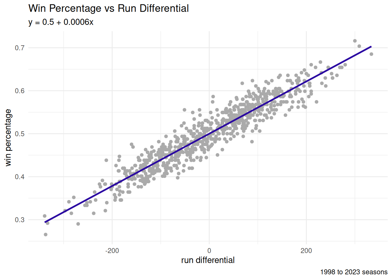
We will proceed by exploring a possible relationship between the run differential and the win percentage.

\[W_{\text{pct}} = \beta_{0} + \beta_{1}*RD + \epsilon\]

In R, we make a linear model using the lm function.

lin_fit <- lm(Wpct ~ RD, data = ch4_data)
lin_fit #print coefficients

## 
## Call:
## lm(formula = Wpct ~ RD, data = ch4_data)
## 
## Coefficients:
## (Intercept)           RD  
##   0.4999841    0.0006081

In ggplot2, we visualize the best-fit line using geom_smooth (with the method = 'lm' parameter).

graph code

ch4_data |>
  ggplot(aes(x = RD, y = Wpct)) +
  geom_point(color = "#AAAAAA") +
  geom_smooth(color = "#2905A1",
              formula = "y ~ x",
              method = "lm",
              se = FALSE) +
  labs(title = "Win Percentage vs Run Differential",
       subtitle = "y = 0.5 + 0.0006x",
       caption = "1998 to 2023 seasons",
       x = "run differential",
       y = "win percentage") +
  theme_minimal() +
  theme(legend.position = "bottom",
        legend.title=element_blank())

\[\beta_{0} = 0.5\]

• \(RD = 0 \rightarrow W_{\text{pct}} = 0.5\)
• Over 162 games: 81 wins

\[\beta_{1} = 0.0006\]

• \(RD = +10 \rightarrow W_{\text{pct}} = 0.506\)
• Over 162 games: 82 wins

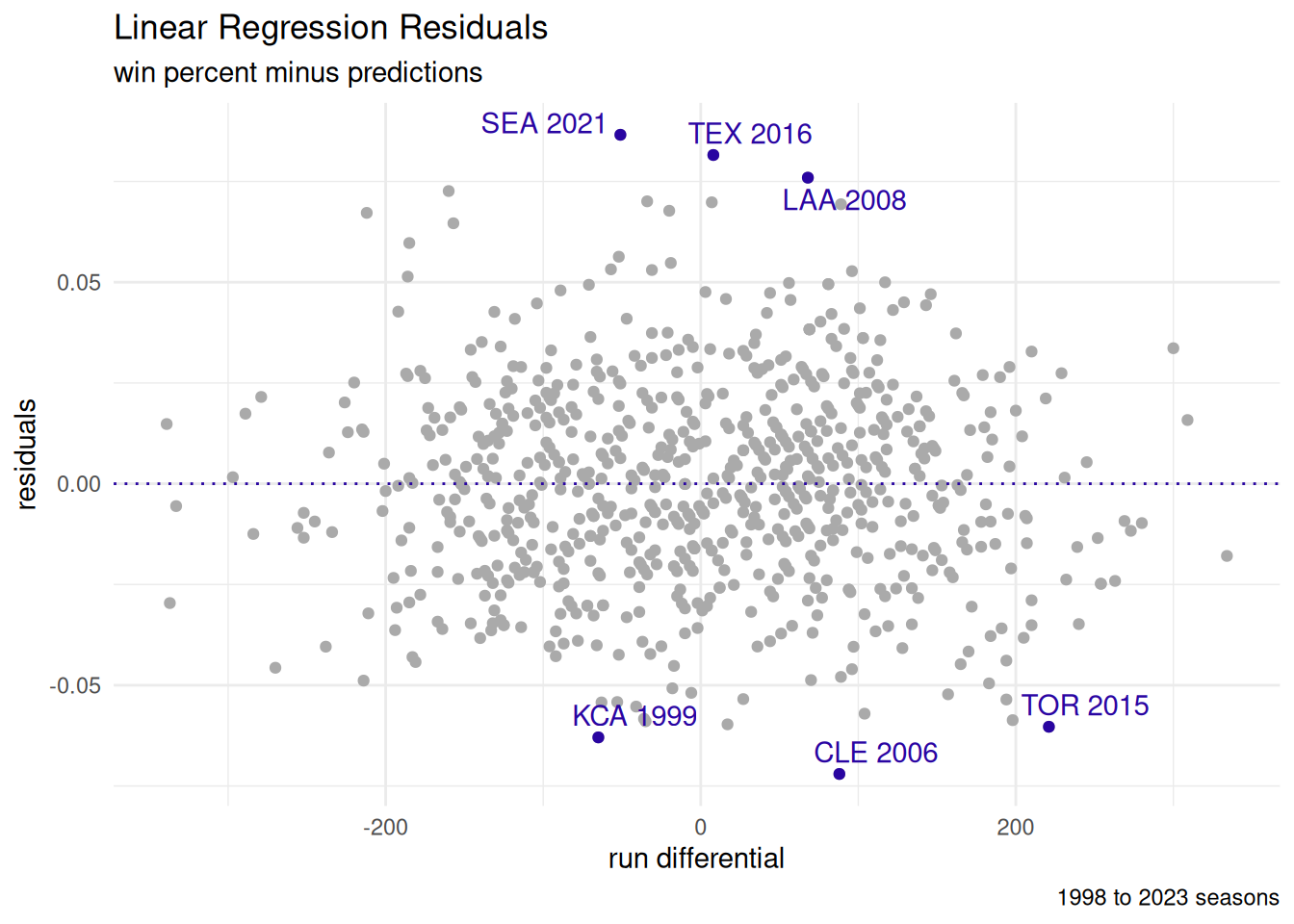
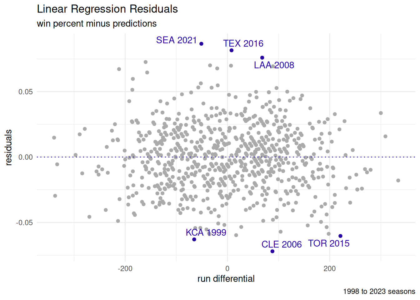
4.5.1 Residuals

Residuals are the differences between the predictions (aka fitted data) and the true values (aka response values).

ch4_data <- ch4_data |>
  mutate(preds = predict(lin_fit, newdata = ch4_data),
         resid = Wpct - preds)

graph code

Residuals
top 3 and bottom 3
teamID	yearID	Wpct	preds	resid	desc
SEA	2021	0.56	0.47	0.09	performed better
TEX	2016	0.59	0.50	0.08	performed better
LAA	2008	0.62	0.54	0.08	performed better
TOR	2015	0.57	0.63	−0.06	performed worse
KCA	1999	0.40	0.46	−0.06	performed worse
CLE	2006	0.48	0.55	−0.07	performed worse

table code

oddities |>
  select(teamID, yearID, Wpct, preds, resid) |>
  mutate(desc = ifelse(resid > 0, "performed better", "performed worse")) |>
  gt() |>
  cols_align(align = "center") |>
  fmt_number(columns = c(Wpct, preds, resid),
             decimals = 2) |>
  tab_header(title = "Residuals",
             subtitle = "top 3 and bottom 3")

4.5.1.1 Balance

For linear models (through least-squares optimization), the average of the residuals should be zero:

mean(ch4_data$resid)

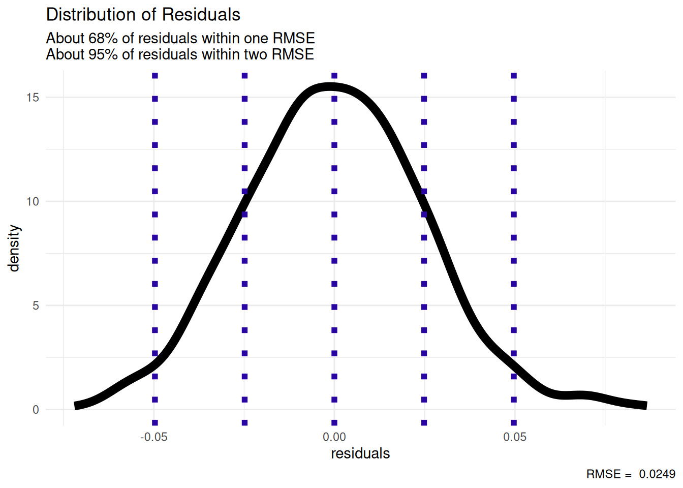
## [1] 1.093195e-16

4.5.1.2 RMSE

The root mean square error acts similarly to a standard deviation to help measure along the variation of our data.

graph code

rmse <- sqrt(mean(ch4_data$resid^2))

ch4_data |>
  ggplot(aes(x = resid)) +
  geom_density(linewidth = 3) +
  geom_vline(color = "#2905A1",
             linetype = 3,
             linewidth = 2,
             xintercept = c(-2*rmse, -1*rmse, 0, rmse, 2*rmse)) +
  labs(title = "Distribution of Residuals",
       subtitle = "About 68% of residuals are within one RMSE\nAbout 95% of residuals are within two RMSE",
       caption = paste("RMSE = ", round(rmse, 4)),
       x = "residuals") +
  theme_minimal()

4.5.2 Discussion

• What about extreme performances?
• Should we relate count statistics to a rate statistic?
• Can we make predictions during the season?