15.6 R code snippetts
Let’s retrieve the titanic_imputed dataset, and the titanic_lmr and titanic_rf models.
titanic_imputed <- archivist::aread("pbiecek/models/27e5c")
titanic_lmr <- archivist::aread("pbiecek/models/58b24")
titanic_rf <- archivist::aread("pbiecek/models/4e0fc")
Construct the explainers
library("rms")
library("randomForest")
library("DALEX")

# explain_lmr <- explain(model = titanic_lmr,
#                        data = titanic_imputed[, -9],
#                        y = titanic_imputed$survived == "yes",
#                        type = "classification",
#                        label = "Logistic Regression")
explain_lmr <- readRDS("./explainers/explain_lmr.rds")

# explain_rf <- explain(model = titanic_rf,
#                       data = titanic_imputed[, -9],
#                       y = titanic_imputed$survived == "yes",
#                       label = "Random Forest")
explain_rf <- readRDS("./explainers/explain_rf.rds")
Function model_performance() calculates, by default, a set of selected model-performance measures.
## Measures for:  classification
## recall     : 0.6385373
## precision  : 0.8832685
## f1         : 0.7412245
## accuracy   : 0.8563661
## auc        : 0.8636533
##
## Residuals:
##      0%     10%     20%     30%     40%     50%     60%     70%     80%     90%
## -0.8920 -0.1140 -0.0240 -0.0080 -0.0040  0.0000  0.0000  0.0100  0.1400  0.5892
##    100%
## 1.0000## Measures for: classification
## recall : 0.5850914
## precision : 0.7522604
## f1 : 0.6582278
## accuracy : 0.8042592
## auc : 0.8174447
##
## Residuals:
## 0% 10% 20% 30% 40% 50%
## -0.98457244 -0.31904861 -0.23408037 -0.20311483 -0.15200813 -0.10318060
## 60% 70% 80% 90% 100%
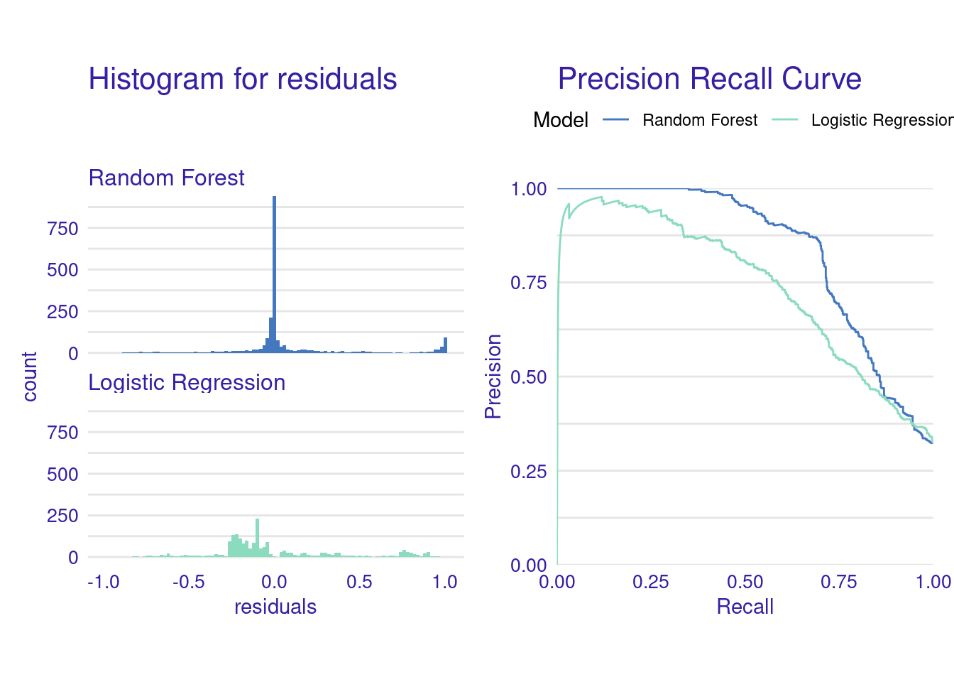
## -0.06933478 0.05858024 0.29306442 0.73666519 0.97151255Plot the residual histograms and precision-recall curves for both models.
library("patchwork")

p1 <- plot(eva_rf, eva_lr, geom = "histogram")
p2 <- plot(eva_rf, eva_lr, geom = "prc")

p1 + p2