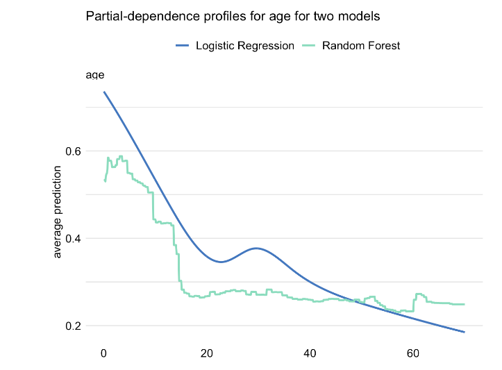
Method
Basic Equations
Mathematical representation of PD profile value for model f(), variable j at value z: \[g_{PD}^{j}(z) = E_{\underline{X}^{-j}}\{f(X^{j|=z})\}\]
where \(\underline{X}^{-j}\) refers to joint distribution of all explanatory variables other than \(X^J\)
We rarely know true distribution of \(\underline{X}^{-j}\), so we typically estimate using the empirical distribution in our training data:
\[\hat g_{PD}^{j}(z) = \frac{1}{n} \sum_{i=1}^{n} f(\underline{x}_i^{j|=z}).\]
The above equation refers to the mean of CP profiles for \(X^J\)
Clustered partial-dependence profiles
- Mean of CP profiles might not be a good representation if profiles are not parallel.
- Alternative approach would be to create multiple clusters of CP profiles:
- Use K-means or hierarchical clustering to identify clusters
- Can use Euclidean distance between CP profiles for identifying similar instances
- Use K-means or hierarchical clustering to identify clusters
Example clustered PDP using rf model on titanic dataset 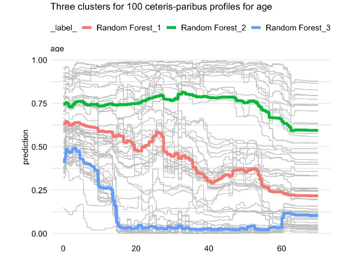
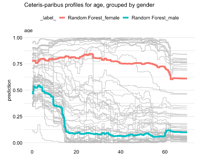
Grouped partial-dependence profiles
- We can use grouped PDPs if we can explicitly identify features that influence the shape of the CP profile for the explanatory variable of interest
- Obvious use case is when model includes interaction between variable of interest and another one.
Example grouped PDP using rf model on titanic dataset