10.3 Example: Titanic imputed dataset

Load packages

suppressPackageStartupMessages({
  library(DALEX)
  library(rms)
  library(randomForest)
  })

Load archivist Titanic imputed dataset, logistic regression and randomg forest models, ‘Henry’ observation.

titanic_imputed <- archivist::aread("pbiecek/models/27e5c")
titanic_lmr <- archivist::aread("pbiecek/models/58b24")
titanic_rf <- archivist::aread("pbiecek/models/4e0fc")
henry <- archivist::aread("pbiecek/models/a6538")

Let’s build two explainers correpsonding to the logistic regresion and random forest models

explain_lmr <- DALEX::explain(model = titanic_lmr, data = titanic_imputed[, -9],
    y = titanic_imputed$survived == "yes", label = "Logistic Regression", verbose = FALSE)

explain_lmr$model_info$type = "classification"

explain_rf <- DALEX::explain(model = titanic_rf,  data = titanic_imputed[, -9],
    y = titanic_imputed$survived == "yes", label = "Random Forest", verbose = FALSE)

Create a CP profiles with ‘Henry’ observation

cp_titanic_rf <- predict_profile(explainer = explain_rf, new_observation = henry)
cp_titanic_lmr <- predict_profile(explainer = explain_lmr, new_observation = henry)

ggplot2::theme_set(theme_ema())

cpplot_age_rf  <- plot(cp_titanic_rf, variables = "age") + 
  ggtitle("Ceteris Paribus for titanic_rf", "") + 
  scale_y_continuous("model response", limits = c(0,1))

cpplot_age_lmr <- plot(cp_titanic_lmr, variables = "age") + 
  ggtitle("Ceteris Paribus for titanic_lmr", "") + 
  scale_y_continuous("model response", limits = c(0,1))

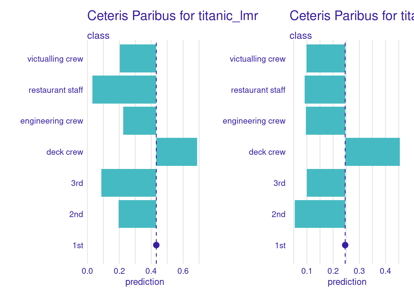
cpplot_class_rf <- plot(cp_titanic_rf, variables = "class", variable_type = "categorical", categorical_type = "bars")  + 
  ggtitle("Ceteris Paribus for titanic_rf", "")

cpplot_class_lmr <- plot(cp_titanic_lmr, variables = "class", variable_type = "categorical", categorical_type = "bars") + 
  ggtitle("Ceteris Paribus for titanic_lmr", "")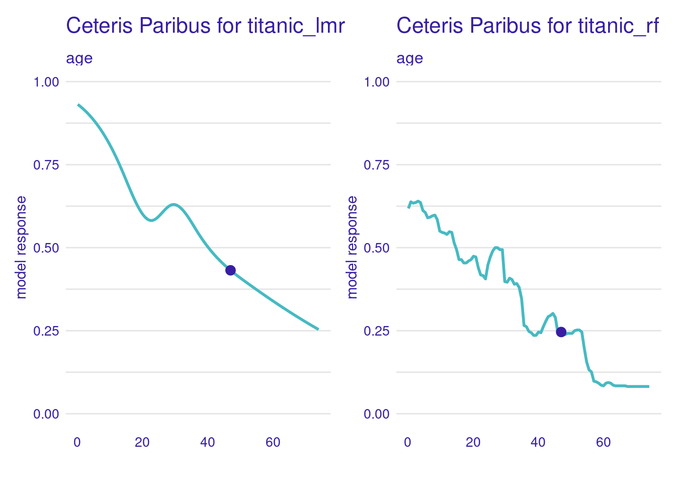

library(patchwork)

cpplot_age_lmr + cpplot_age_rf

Both CP profiles predict the survival probability for passenger Henry (1st class, age = 47, male), where the logistic regression results in 0.43 and the random forest model is 0.246.

cpplot_class_lmr + cpplot_class_rf

Both models agree on the prediction direction, but not on the vector magnitude.

plot(cp_titanic_rf) + 
  facet_wrap(~`_vname_`, ncol = 4, scales = "free_x") + 
  ggtitle("Ceteris Paribus for titanic_rf", "")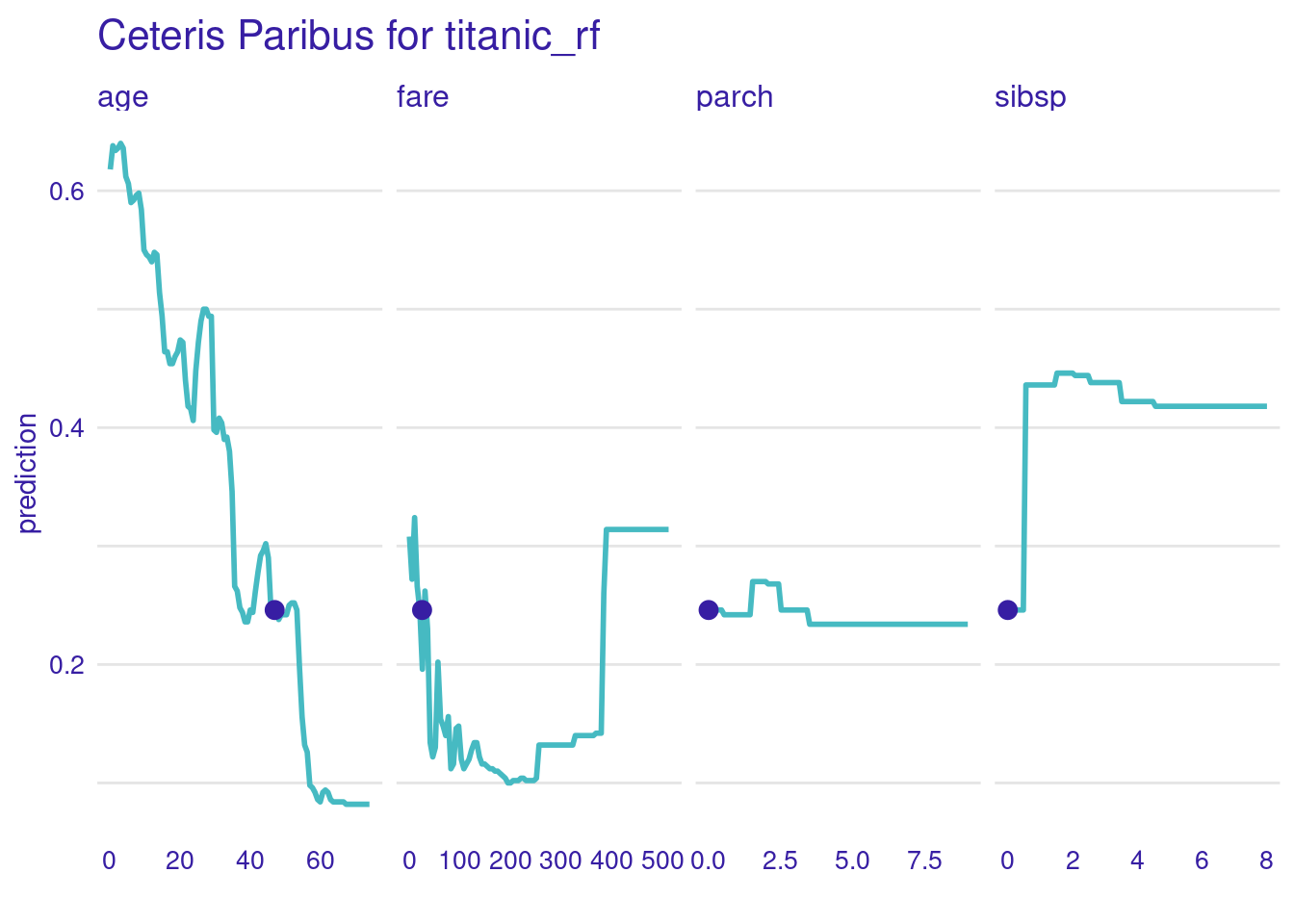

CP profiles for all continuous variables. What can we infer from the behavior of these variables?