9.2 Method
Loss Function Minimization
\[ \hat g = \arg \min_{g \in \mathcal{G}} L\{f, g, \nu(\underline{x}_*)\} + \Omega (g), \] where
- \(\mathcal{G}\) is class of simple models
- \(f\) is black box model prediction
- \(g\) is glass box model prediction
- \(\nu(\underline{x}_*)\) is neighborhood around instance \(\underline{x}_*\)
- \(\Omega (g)\) is penalty for complexity of \(f\)
In practice, exclude \(\Omega (g)\) from optimization procedure. Instead, manually control complexity by specifying number of coefficients in glass-box model.
f() and g() operate on different spaces:
- f() works in \(p\) dimensions, corresponds to \(p\) predictors
- g() corresponds to \(q\) dimensional spaces
- \(q << p\)
Glass-box Fitting Procedure
Specify:
  - x* instance of interest
  - N sample size of artificial points
  - K number of predictor variables for glass-box model
  - similarity function
  - glass box model

Steps:
1. Sample N artificial points around instance.
2. Fit black box model to points -- becomes target variable
3. Calculate similarity between instance and each artifical point
4. Fit glass box model:
    -use N artificial points as features
    -use black-box predictions on N points as target
    -limit to K nonzero coefficients
    -Weight training of each point using similarity measure
Image Classifier Example
Overview:
- Classify 244 x 244 color image into 1,000 potential categories
- Goal: Explain model classification.
- Issue: High dimensional problem: Each image comprises 178,608 dimensions (3 x 244 x 244)
Solution:
- Transform into 100 superpixels. Glass box applies to \(\{0,1\}^{100}\) space
- Sample around instance - (i.e.,randomly exclude some superpxiels)
- Fit LASSO with K=15 nonzero coefficients
![]()
Figure 9.3: Left-original image; Middle-superpixels; Right-artificial data
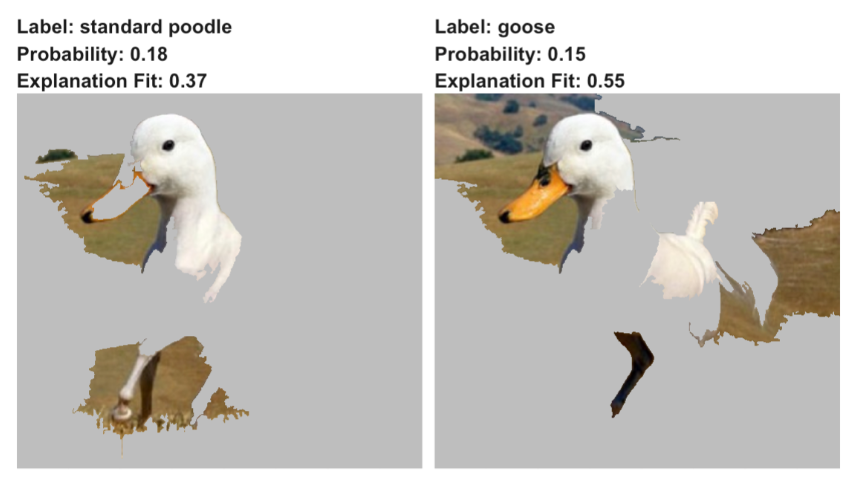
Figure 9.4: 15 selected superpixel features
Sampling around instance
- Can’t always sample from existing points because data very sparse and “far” from each other in high dimensional space
- Usually instead create perturbations on instance of interest
- continuous variables - multiple approaches
- adding Gaussian noise
- perturb discretized versions of of variables
- adding Gaussian noise
- binary variables - change some 0s to 1s and vice-versa
- continuous variables - multiple approaches