9.5 Code Examples in R

Package options

• lime is port of Python library, discretizes variables based on quartiles
  
• localModel uses ceteris-paribus profiles,
• iml works directly on continuous variables. One of package authors wrote popular interpretable ML book

Notes:

• DALExtra package needed for predict_surrogate() interface to multiple packages.
  
• Default method ofpredict_surrogate() is localModel.
  
• Examples below use K-LASSO for glass-box model

# core libraries
library(randomForest)
library(DALEX)
library(DALEXtra)

# load data nd models 
titanic_imputed <- archivist::aread("pbiecek/models/27e5c")
titanic_rf <- archivist:: aread("pbiecek/models/4e0fc")
johnny_d <- archivist:: aread("pbiecek/models/e3596")  

# explainer
titanic_rf_exp <- DALEX::explain(model = titanic_rf,  
                        data = titanic_imputed[, -9],
                           y = titanic_imputed$survived == "yes", 
                       label = "Random Forest")

## Preparation of a new explainer is initiated
##   -> model label       :  Random Forest 
##   -> data              :  2207  rows  8  cols 
##   -> target variable   :  2207  values 
##   -> predict function  :  yhat.randomForest  will be used (  default  )
##   -> predicted values  :  No value for predict function target column. (  default  )
##   -> model_info        :  package randomForest , ver. 4.7.1.1 , task classification (  default  ) 
##   -> model_info        :  Model info detected classification task but 'y' is a logical . Converted to numeric.  (  NOTE  )
##   -> predicted values  :  numerical, min =  0 , mean =  0.2353095 , max =  1  
##   -> residual function :  difference between y and yhat (  default  )
##   -> residuals         :  numerical, min =  -0.892 , mean =  0.0868473 , max =  1  
##   A new explainer has been created!

Package: lime

Fit model:

library(lime)
set.seed(1)

# lime model
model_type.dalex_explainer <- DALEXtra::model_type.dalex_explainer
predict_model.dalex_explainer <- DALEXtra::predict_model.dalex_explainer

lime_johnny <- predict_surrogate(explainer = titanic_rf_exp, 
                  new_observation = johnny_d, 
                  n_features = 3, 
                  n_permutations = 1000,
                  type = "lime")

model_type	case	model_r2	model_intercept	model_prediction	feature	feature_value	feature_weight	feature_desc	data	prediction
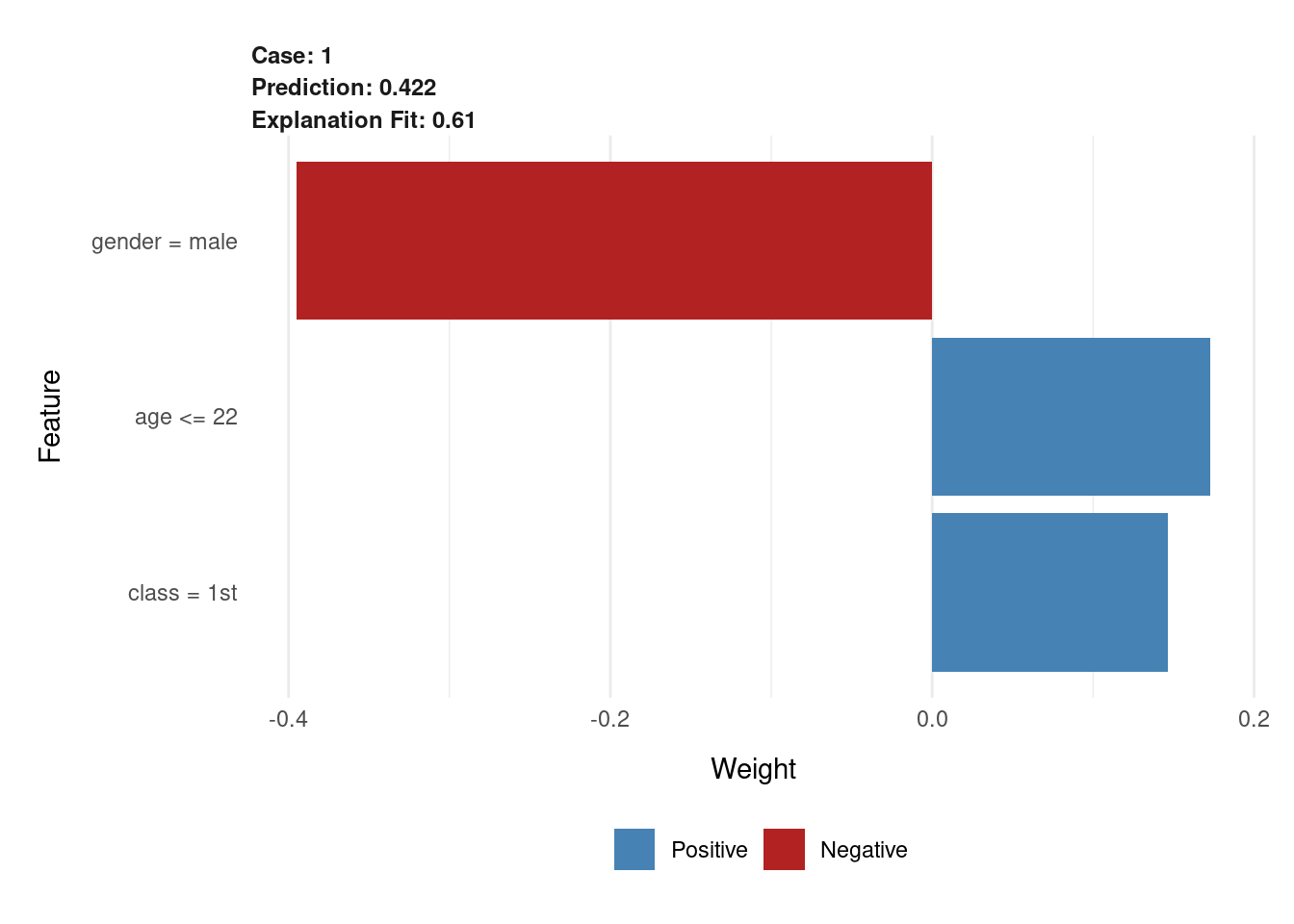
regression	1	0.613	0.557	0.481	gender	2	-0.395	gender = male	2, 8, 1, 4, 72, 0, 0	0.422
regression	1	0.613	0.557	0.481	age	8	0.173	age <= 22	2, 8, 1, 4, 72, 0, 0	0.422
regression	1	0.613	0.557	0.481	class	1	0.146	class = 1st	2, 8, 1, 4, 72, 0, 0	0.422

Interpretable equation:

\[ \hat p_{lime} = 0.557 - 0.395 \cdot 1_{male} + 0.173 \cdot 1_{age <= 22} + 0.146 \cdot 1_{class = 1st}=0.481, \] Plot lime model:

plot(lime_johnny)

Package: localModel

library(localModel)

# localModel build
locMod_johnny <- predict_surrogate(explainer = titanic_rf_exp, 
                  new_observation = johnny_d, 
                  size = 1000,
                  seed = 1,
                  type = "localModel")

estimated	variable	original_variable
0.235	(Model mean)
0.619	(Intercept)
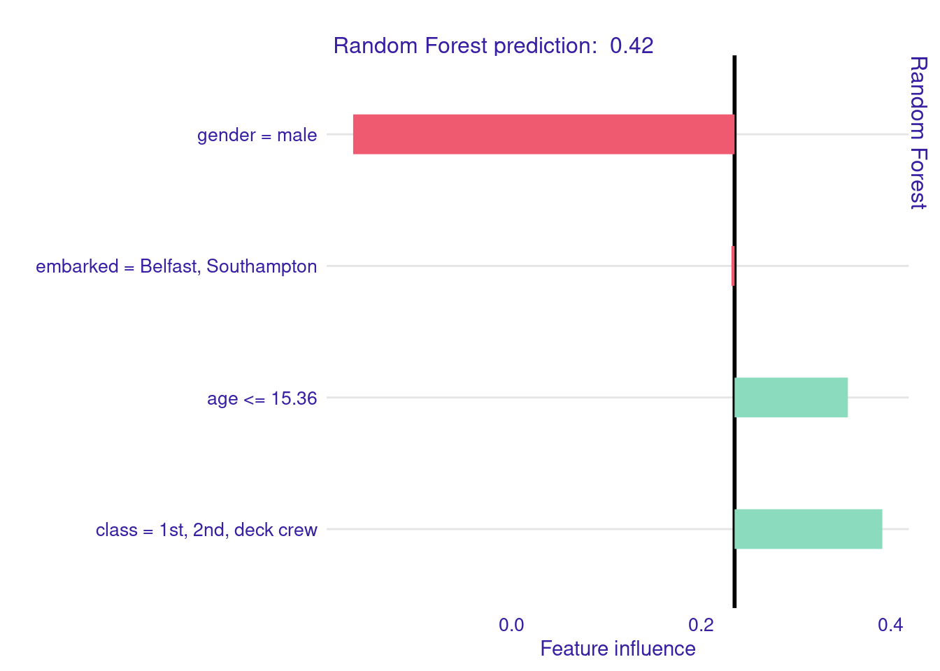
-0.402	gender = male	gender
0.120	age <= 15.36	age
0.156	class = 1st, 2nd, deck crew	class
-0.003	embarked = Belfast, Southampton	embarked

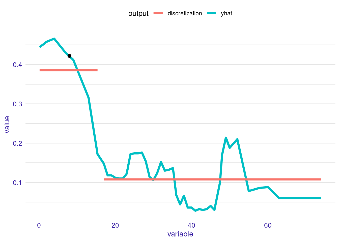
Plot to explain how continuous age variable was dichotomized:

# plot
plot_interpretable_feature(locMod_johnny, "age")

Glass-box explanation plot for Johnny D:

plot(locMod_johnny)

Package: iml

library(iml)

# model using iml pacakge
iml_johnny <- predict_surrogate(explainer = titanic_rf_exp, 
                  new_observation = johnny_d, 
                  k = 3, 
                  type = "iml",
                  seed=1)

beta	x.recoded	effect	x.original	feature	.class
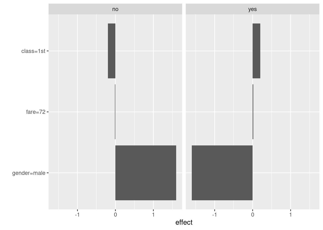
0.199	1	0.199	1st	class=1st	yes
-1.601	1	-1.601	male	gender=male	yes
0.000	72	0.015	72	fare	yes

Notes:

• continuous variables are not transformed
  
• categorical variables dichotomized with value 1 for observed category; otherwise 0

Glass-box explanation plot for Johnny D:

plot(iml_johnny)

The age, gender and class are correlated, and may partially explain why explanations are somewhat different across various LIME implementations.