4.1 Selecting multiple elements
4.1.1 Atomic Vectors
- 6 ways to subset atomic vectors
Let’s take a look with an example vector.
Positive integer indices
# return elements at specified positions which can be out of order
x[c(4, 1)]
#> [1] 4.4 1.1

# duplicate indices return duplicate values
x[c(2, 2)]
#> [1] 2.2 2.2

# real numbers truncate to integers
# so this behaves as if it is x[c(3, 3)]
x[c(3.2, 3.8)]
#> [1] 3.3 3.3
Negative integer indices
### excludes elements at specified positions
x[-c(1, 3)] # same as x[c(-1, -3)] or x[c(2, 4)]
#> [1] 2.2 4.4

### mixing positive and negative is a no-no
x[c(-1, 3)]
#> Error in x[c(-1, 3)]: only 0's may be mixed with negative subscripts
Logical Vectors
x[c(TRUE, TRUE, FALSE, TRUE)]
#> [1] 1.1 2.2 4.4

x[x < 3]
#> [1] 1.1 2.2

cond <- x > 2.5
x[cond]
#> [1] 3.3 4.4- Recyling rules applies when the two vectors are of different lengths
- the shorter of the two is recycled to the length of the longer
- Easy to understand if x or y is 1, best to avoid other lengths
Missing values (NA)
Nothing
Zero
Character vectors
# if name, you can use to return matched elements
(y <- setNames(x, letters[1:4]))
#>   a   b   c   d
#> 1.1 2.2 3.3 4.4

y[c("d", "b", "a")]
#>   d   b   a
#> 4.4 2.2 1.1

# Like integer indices, you can repeat indices
y[c("a", "a", "a")]
#>   a   a   a
#> 1.1 1.1 1.1

# When subsetting with [, names are always matched exactly
z <- c(abc = 1, def = 2)
z
#> abc def
#>   1   2
z[c("a", "d")]
#> <NA> <NA>
#>   NA   NA
4.1.2 Lists
- Subsetting works the same way
[always returns a list[[and$let you pull elements out of a list
my_list <- list(a = c(T, F), b = letters[5:15], c = 100:108)
my_list
#> $a
#> [1]  TRUE FALSE
#>
#> $b
#>  [1] "e" "f" "g" "h" "i" "j" "k" "l" "m" "n" "o"
#>
#> $c
#> [1] 100 101 102 103 104 105 106 107 108
Return a (named) list
Return a vector
l2 <- my_list[[2]]
l2
#>  [1] "e" "f" "g" "h" "i" "j" "k" "l" "m" "n" "o"
l2b <- my_list$b
l2b
#>  [1] "e" "f" "g" "h" "i" "j" "k" "l" "m" "n" "o"
Return a specific element
l3 <- my_list[[2]][3]
l3
#> [1] "g"
l4 <- my_list[['b']][3]
l4
#> [1] "g"
l4b <- my_list$b[3]
l4b
#> [1] "g"
Visual Representation
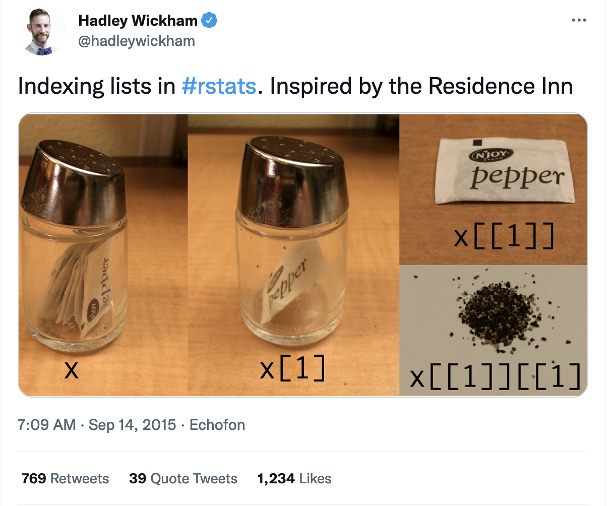
See this stackoverflow article for more detailed information about the differences: https://stackoverflow.com/questions/1169456/the-difference-between-bracket-and-double-bracket-for-accessing-the-el
4.1.3 Matrices and arrays
You can subset higher dimensional structures in three ways:
- with multiple vectors
- with a single vector
- with a matrix
a <- matrix(1:12, nrow = 3)
colnames(a) <- c("A", "B", "C", "D")

# single row
a[1, ]
#>  A  B  C  D
#>  1  4  7 10

# single column
a[, 1]
#> [1] 1 2 3

# single element
a[1, 1]
#> A
#> 1

# two rows from two columns
a[1:2, 3:4]
#>      C  D
#> [1,] 7 10
#> [2,] 8 11

a[c(TRUE, FALSE, TRUE), c("B", "A")]
#>      B A
#> [1,] 4 1
#> [2,] 6 3

# zero index and negative index
a[0, -2]
#>      A C D
Subset a matrix with a matrix
vals <- outer(1:5, 1:5, FUN = "paste", sep = ",")
vals
#>      [,1]  [,2]  [,3]  [,4]  [,5]
#> [1,] "1,1" "1,2" "1,3" "1,4" "1,5"
#> [2,] "2,1" "2,2" "2,3" "2,4" "2,5"
#> [3,] "3,1" "3,2" "3,3" "3,4" "3,5"
#> [4,] "4,1" "4,2" "4,3" "4,4" "4,5"
#> [5,] "5,1" "5,2" "5,3" "5,4" "5,5"

select <- matrix(ncol = 2, byrow = TRUE,
                 c(1, 1,
                   3, 1,
                   2, 4))
select
#>      [,1] [,2]
#> [1,]    1    1
#> [2,]    3    1
#> [3,]    2    4

vals[select]
#> [1] "1,1" "3,1" "2,4"
Matrices and arrays are just special vectors; can subset with a single vector (arrays in R stored column wise)
4.1.4 Data frames and tibbles
Data frames act like both lists and matrices
- When subsetting with a single index, they behave like lists and index the columns, so
df[1:2]selects the first two columns. - When subsetting with two indices, they behave like matrices, so
df[1:3, ]selects the first three rows (and all the columns).
library(palmerpenguins)
penguins <- penguins

# single index selects first two columns
two_cols <- penguins[2:3] # or penguins[c(2,3)]
head(two_cols)
#> # A tibble: 6 × 2
#>   island    bill_length_mm
#>   <fct>              <dbl>
#> 1 Torgersen           39.1
#> 2 Torgersen           39.5
#> 3 Torgersen           40.3
#> 4 Torgersen           NA
#> 5 Torgersen           36.7
#> 6 Torgersen           39.3

# equivalent to the above code
same_two_cols <- penguins[c("island", "bill_length_mm")]
head(same_two_cols)
#> # A tibble: 6 × 2
#>   island    bill_length_mm
#>   <fct>              <dbl>
#> 1 Torgersen           39.1
#> 2 Torgersen           39.5
#> 3 Torgersen           40.3
#> 4 Torgersen           NA
#> 5 Torgersen           36.7
#> 6 Torgersen           39.3

# two indices separated by comma (first two rows of 3rd and 4th columns)
penguins[1:2, 3:4]
#> # A tibble: 2 × 2
#>   bill_length_mm bill_depth_mm
#>            <dbl>         <dbl>
#> 1           39.1          18.7
#> 2           39.5          17.4

# Can't do this...
penguins[[3:4]][c(1:4)]
#> Error:
#> ! The `j` argument of `[[.tbl_df()` can't be a vector of length 2 as of
#>   tibble 3.0.0.
#> ℹ Recursive subsetting is deprecated for tibbles.
# ...but this works...
penguins[[3]][c(1:4)]
#> [1] 39.1 39.5 40.3   NA
# ...or this equivalent...
penguins$bill_length_mm[1:4]
#> [1] 39.1 39.5 40.3   NA
Subsetting a tibble with [ always returns a tibble
4.1.5 Preserving dimensionality
- Data frames and tibbles behave differently
- tibble will default to preserve dimensionality, data frames do not
- this can lead to unexpected behavior and code breaking in the future
- Use
drop = FALSEto preserve dimensionality when subsetting a data frame or use tibbles
tb <- tibble::tibble(a = 1:2, b = 1:2)

# returns tibble
str(tb[, "a"])
#> tibble [2 × 1] (S3: tbl_df/tbl/data.frame)
#>  $ a: int [1:2] 1 2
tb[, "a"] # equivalent to tb[, "a", drop = FALSE]
#> # A tibble: 2 × 1
#>       a
#>   <int>
#> 1     1
#> 2     2

# returns integer vector
# str(tb[, "a", drop = TRUE])
tb[, "a", drop = TRUE]
#> [1] 1 2
df <- data.frame(a = 1:2, b = 1:2)
# returns integer vector
# str(df[, "a"])
df[, "a"]
#> [1] 1 2
# returns data frame with one column
# str(df[, "a", drop = FALSE])
df[, "a", drop = FALSE]
#> a
#> 1 1
#> 2 2Factors
Factor subsetting drop argument controls whether or not levels (rather than dimensions) are preserved.