3.5 Class - S3 atomic vectors
Credit: Advanced R by Hadley Wickham
Having a class attribute turns an object into an S3 object.
What makes S3 atomic vectors different?
- behave differently from a regular vector when passed to a generic function
- often store additional information in other attributes
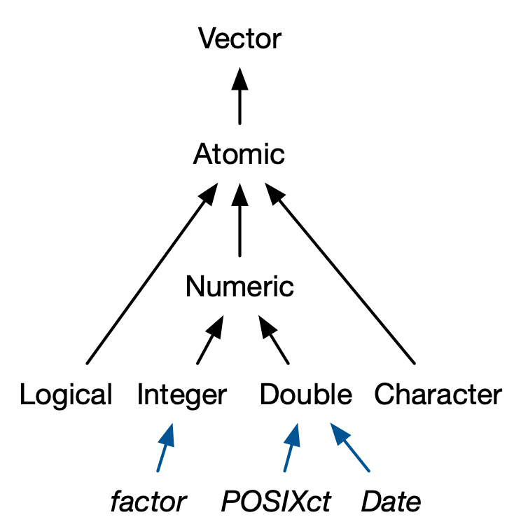
Four important S3 vectors used in base R:
- Factors (categorical data)
- Dates
- Date-times (POSIXct)
- Durations (difftime)
3.5.1 Factors
A factor is a vector used to store categorical data that can contain only predefined values.
Factors are integer vectors with:
- Class: “factor”
- Attributes: “levels”, or the set of allowed values
colors = c('red', 'blue', 'green','red','red', 'green')
# Build a factor
a_factor <- factor(
  # values
  x = colors,
  # exhaustive list of values
  levels = c('red', 'blue', 'green', 'yellow')
)
# Useful when some possible values are not present in the data
table(colors)
#> colors
#> blue green red
#> 1 2 3
table(a_factor)
#> a_factor
#> red blue green yellow
#> 3 1 2 0
# - type
typeof(a_factor)
#> [1] "integer"
class(a_factor)
#> [1] "factor"
# - attributes
attributes(a_factor)
#> $levels
#> [1] "red" "blue" "green" "yellow"
#>
#> $class
#> [1] "factor"3.5.1.1 Custom Order
Factors can be ordered. This can be useful for models or visualizations where order matters.
values <- c('high', 'med', 'low', 'med', 'high', 'low', 'med', 'high')

ordered_factor <- ordered(
  # values
  x = values,
  # levels in ascending order
  levels = c('low', 'med', 'high')
)

# Inspect
ordered_factor
#> [1] high med  low  med  high low  med  high
#> Levels: low < med < high

table(values)
#> values
#> high  low  med
#>    3    2    3
table(ordered_factor)
#> ordered_factor
#>  low  med high
#>    2    3    3
3.5.2 Dates
Dates are:
- Double vectors
- With class “Date”
- No other attributes
notes_date <- Sys.Date()

# type
typeof(notes_date)
#> [1] "double"

# class
attributes(notes_date)
#> $class
#> [1] "Date"
The double component represents the number of days since since the Unix epoch 1970-01-01
3.5.3 Date-times
There are 2 Date-time representations in base R:
- POSIXct, where “ct” denotes calendar time
- POSIXlt, where “lt” designates local time
We’ll focus on POSIXct because:
- Simplest
- Built on an atomic (double) vector
- Most appropriate for use in a data frame
Let’s now build and deconstruct a Date-time
# Build
note_date_time <- as.POSIXct(
  x = Sys.time(), # time
  tz = "America/New_York" # time zone, used only for formatting
)

# Inspect
note_date_time
#> [1] "2024-11-09 10:16:54 EST"

# - type
typeof(note_date_time)
#> [1] "double"

# - attributes
attributes(note_date_time)
#> $class
#> [1] "POSIXct" "POSIXt"
#>
#> $tzone
#> [1] "America/New_York"

structure(note_date_time, tzone = "Europe/Paris")
#> [1] "2024-11-09 16:16:54 CET"3.5.4 Durations
Durations represent the amount of time between pairs of dates or date-times.
- Double vectors
- Class: “difftime”
- Attributes: “units”, or the unit of duration (e.g., weeks, hours, minutes, seconds, etc.)
# Construct
one_minute <- as.difftime(1, units = "mins")
# Inspect
one_minute
#> Time difference of 1 mins

# Dissect
# - type
typeof(one_minute)
#> [1] "double"
# - attributes
attributes(one_minute)
#> $class
#> [1] "difftime"
#>
#> $units
#> [1] "mins"See also:
3.5.5 Exercises
- What sort of object does
table()return? What is its type? What attributes does it have? How does the dimensionality change as you tabulate more variables?
Answer(s)
table() returns a contingency table of its input variables. It is implemented as an integer vector with class table and dimensions (which makes it act like an array). Its attributes are dim (dimensions) and dimnames (one name for each input column). The dimensions correspond to the number of unique values (factor levels) in each input variable.
- What happens to a factor when you modify its levels?
Answer(s)
The underlying integer values stay the same, but the levels are changed, making it look like the data has changed.
f1 <- factor(letters)
f1
#>  [1] a b c d e f g h i j k l m n o p q r s t u v w x y z
#> Levels: a b c d e f g h i j k l m n o p q r s t u v w x y z
as.integer(f1)
#>  [1]  1  2  3  4  5  6  7  8  9 10 11 12 13 14 15 16 17 18 19 20 21 22 23 24 25
#> [26] 26

levels(f1) <- rev(levels(f1))
f1
#>  [1] z y x w v u t s r q p o n m l k j i h g f e d c b a
#> Levels: z y x w v u t s r q p o n m l k j i h g f e d c b a
as.integer(f1)
#>  [1]  1  2  3  4  5  6  7  8  9 10 11 12 13 14 15 16 17 18 19 20 21 22 23 24 25
#> [26] 26- What does this code do? How do
f2andf3differ fromf1?
Answer(s)
For f2 and f3 either the order of the factor elements or its levels are being reversed. For f1 both transformations are occurring.
# Reverse element order
(f2 <- rev(factor(letters)))
#>  [1] z y x w v u t s r q p o n m l k j i h g f e d c b a
#> Levels: a b c d e f g h i j k l m n o p q r s t u v w x y z
as.integer(f2)
#>  [1] 26 25 24 23 22 21 20 19 18 17 16 15 14 13 12 11 10  9  8  7  6  5  4  3  2
#> [26]  1

# Reverse factor levels (when creating factor)
(f3 <- factor(letters, levels = rev(letters)))
#>  [1] a b c d e f g h i j k l m n o p q r s t u v w x y z
#> Levels: z y x w v u t s r q p o n m l k j i h g f e d c b a
as.integer(f3)
#>  [1] 26 25 24 23 22 21 20 19 18 17 16 15 14 13 12 11 10  9  8  7  6  5  4  3  2
#> [26]  1