10.4.2 Theme, Legends and Guides

• Use theme to customise non-data elements of a plot.

• Many built-in themes.

• Create your own theme and save as a template.

• Change default theme with theme_set() function.

theme_scatter <- function(base_size = 14) {
  theme_bw(base_size = base_size) %+replace%
    theme(
      axis.line = element_line(colour = "black"),
      plot.background = element_blank(),
      panel.grid.major = element_blank(),
      panel.grid.minor = element_blank(),
      panel.border = element_blank(),
      text = element_text(family = "sans",
                          size = 12),
      axis.text = element_text(colour = "black")
    )
}

scatter +
  theme_scatter()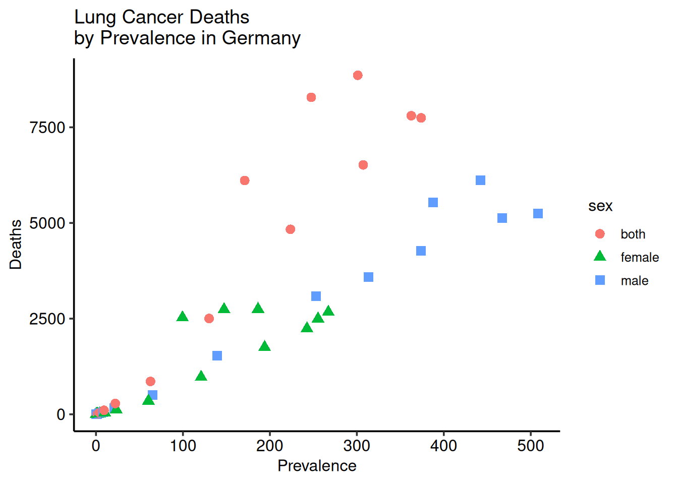

• The use of %+replace% replaces theme elements.

• guides and guide can be used with scale to fine-tune plot design and layout.

# Customising a legend to a plot
lineplot1 <- lineplot +
  labs(
    linetype = "Sex",
    subtitle = "Year 2019",
    caption = "DataSource: hmsidwR::germany_lungc"
  ) +
  guides(linetype = guide_legend(reverse = TRUE)) +
  theme_classic() +
  theme(
    legend.position = "top",
    axis.text.x = element_text(angle = 45, hjust = 1),
    plot.title = element_text(hjust = 0.5, face = "bold")
  )

lineplot1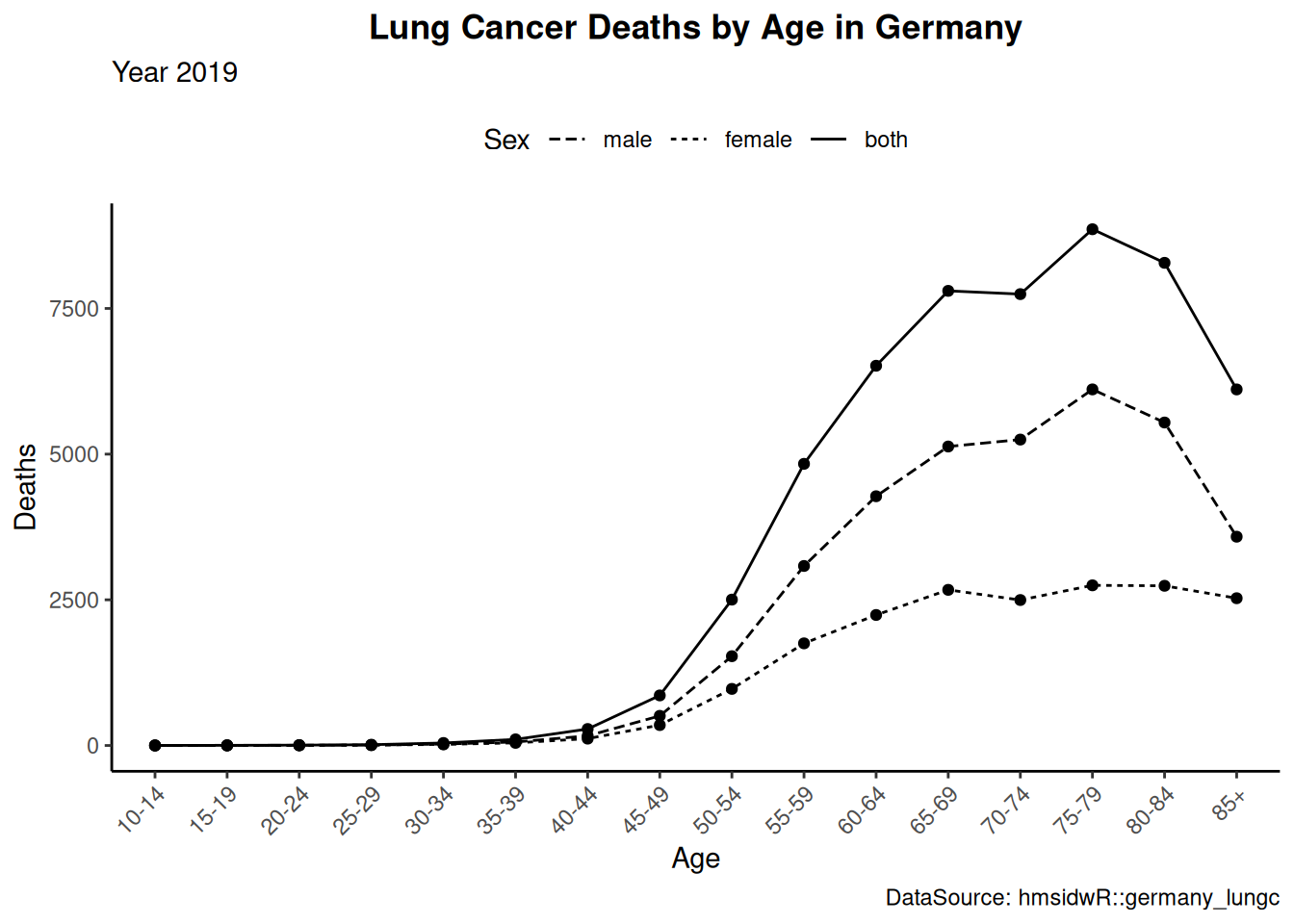

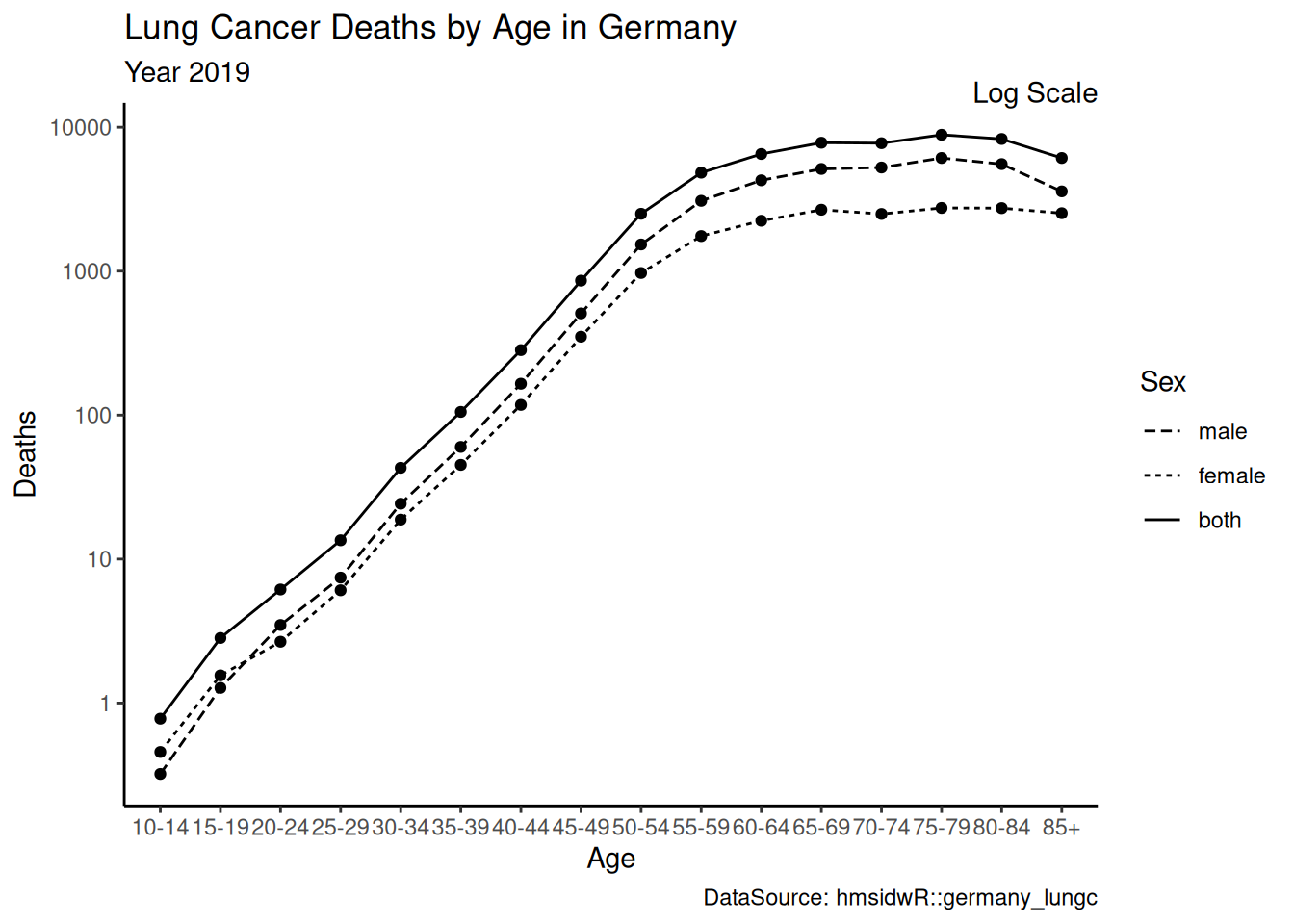
lineplot2 <- lineplot1 + 
  
  # Apply a log base 10 scale to the y axis
  scale_y_log10() + 
  
  # Allows for the drawing of data points anywhere on the plot
  coord_cartesian(clip = "off") +
  annotate("text", x = Inf, y=Inf, 
           hjust = 1, vjust = 0,
           label = "Log Scale") +
  theme_classic()

lineplot2