7.3 Case Study: Predicting Rabies
7.3.1 Goal:
Predict DALYs due to rabies in ‘Asia’ and ‘Global’ regions, using the hmsidwR::rabies dataset
7.3.2 Exploratory Data Analysis (EDA)
Dataset contains all cause and rabies mortality plus DALYs for the Asian and Global region, subdivided by year
Values have an estimate and upper and lower boundaries in separate columns
240 observations across 7 variables.
Examining the data shows that death rates (
dx_rabies) and DALYs (dalys_rabies) are different in magnitude and scale
library(tidyverse)
rabies <- hmsidwR::rabies %>%
  filter(year >= 1990 & year <= 2019) %>%
  select(-upper, -lower) %>%
  pivot_wider(names_from = measure, values_from = val) %>%
  filter(cause == "Rabies") %>%
  rename(dx_rabies = Deaths, dalys_rabies = DALYs) %>%
  select(-cause)

rabies %>% head()
## # A tibble: 6 × 4
## location year dx_rabies dalys_rabies
## <chr> <dbl> <dbl> <dbl>
## 1 Asia 1990 0.599 33.1
## 2 Asia 1992 0.575 31.9
## 3 Asia 1994 0.554 30.7
## 4 Asia 1991 0.585 32.3
## 5 Asia 1995 0.551 30.5
## 6 Asia 1997 0.502 27.9- After scaling, these values are closer together in magnitude, avoiding the issue of larger variables dominating others in prediction
library(patchwork)

p1 <- rabies %>%
  ggplot(aes(x = year, group = location, linetype = location)) +
  geom_line(aes(y = dx_rabies),
            linewidth = 1) +
  geom_line(aes(y = dalys_rabies))

p2 <- rabies %>%
  # apply a scale transformation to the numeric variables
  mutate(year = as.integer(year),
         across(where(is.double), scale)) %>%
  ggplot(aes(x = year, group = location, linetype = location)) +
  geom_line(aes(y = dx_rabies),
            linewidth = 1) +
  geom_line(aes(y = dalys_rabies))

p1 + p2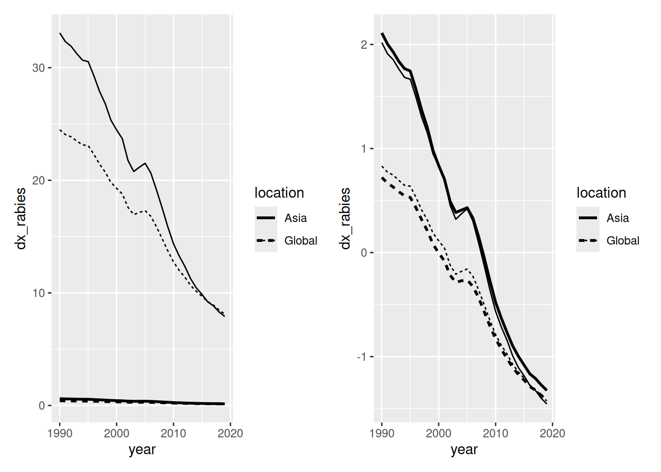
7.3.3 Training and Resampling
- The dataset was split into 80% training and 20% final test, stratified by location
- The 80% training set was then used to create a series of ‘folds’ or resamples of the data
- These folds can then be used to validate how well each model (and selected parameters) match unseen data
- K-fold cross validation was used to generate 10 folds using the
vfold_cv()function from the tidymodels package
7.3.4 Preprocessing
- Handled using ‘recipes’ as part of tidymodels pipelines
- Recipe 0 - all predictors, no transformations [reference model]
- Recipe 1 - encoding of dummy variable for region, standardised numeric variables
- Recipe 2 - as recipe 2, with addition of method to reduce skewness of
dalys_rabiesoutcome - Advantage of ‘recipe’ approach in tidymodels is that they can be piped / swapped out easily.
7.3.5 Multicollinearity
- DALYs & mortality likely to be strongly correlated (DALYs = Years_life_lost + Years_lived_w_disability))
- All cause and specific cause mortality also will have some correlation
- This can cause issues with some prediction methods, making it hard for the model to determine which variables have the best predictive power.
- In this analysis, dealt with by the choice of prediction method: Random forests and GLM with lasso penalty both robust to multicollinearity
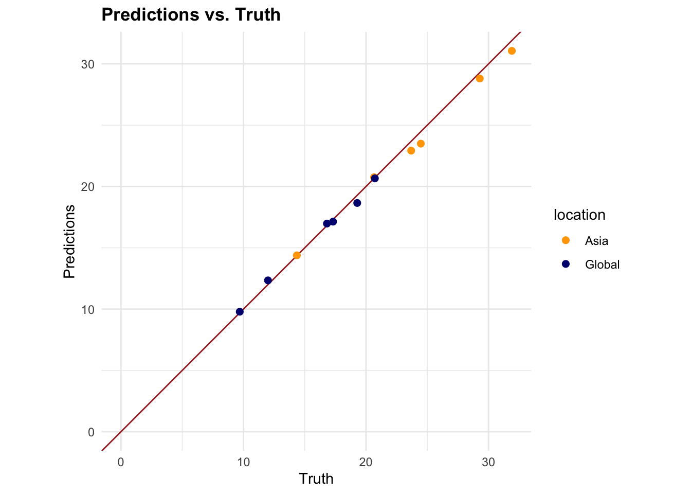
7.3.6 Model 1: Random forest
- Specified using
rand_forest()function within tidymodels framework - Hyperparameters tuned using cross-validation and
tune_grid()/ grid search - Optimal parameters gave RMSE 0.506
- Fig 7.4a shows close relationship between predictions and observed data