12.6 Dynamics of Disease Transmission
Disease transmission can be modelled using various approaches, including:
- Compartmental models (e.g., SIR, SEIR)
- Agent-based models
- Network models
12.6.1 Spatial Proximity with Kriging
Kriging is a geostatistical method used to predict the value of a variable at unsampled locations based on the values at sampled locations. It is particularly useful for spatial data with spatial correlation.
set.seed(21082024) # set seed for reproducibility
num_points <- 100
# simulate the presence of infection
# 1 = "infected" and 0 = "non_infected"
longitude <- rnorm(n = num_points, mean = 20.70, sd = 1)
latitude <-  rnorm(n = num_points, mean = 6.294, sd = 1)
presence <- rbinom(100, 1, prob = 0.3)
cases <- ifelse(presence == 1,
                rpois(n = num_points*0.7, lambda = 10), 0)
temperature <- rnorm(n = num_points,
                     mean = 24.7,
                     sd = (29.2 - 20.3) / 4)

# build a dataframe
df <- data.frame(longitude, latitude,
                 presence, cases, temperature)

df_sf <- df %>%
  st_as_sf(coords = c("longitude","latitude"),
           # or use crs = 4326
           crs = "+proj=longlat +datum=WGS84") %>%
  st_intersection(ctr_africa) %>%
st_make_valid()library(gstat)
v <- variogram(object = cases ~ temperature, data = df_sf)
v_model <- fit.variogram(v, model = vgm("Sph"))
plot(v, model = v_model)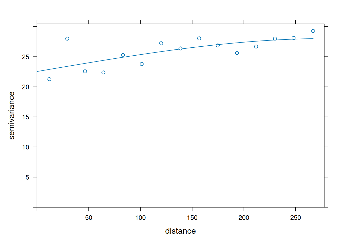
12.6.2 Perform Kriging
to predict the spatial distribution of the variable of interest (e.g., temperature) across a grid of points in Central African Republic.
library(DescTools)
set.seed(240724) # set seed for reproducibility
ctr_africa_coords <- ctr_africa %>%
  sf::st_coordinates() %>%
  as.data.frame() %>%
  dplyr::select(X, Y)
bbox <- ctr_africa %>% st_bbox()
bbox_grid <- expand_grid(x = seq(from = bbox$xmin,
                                 to = bbox$xmax,
                                 length.out = 100),
                         y = seq(from = bbox$ymin,
                                 to = bbox$ymax,
                                 length.out = 100))

ctr_africa_grid_full <- data.frame(PtInPoly(bbox_grid,
                                            ctr_africa_coords))

ctr_africa_grid <- ctr_africa_grid_full %>%
  filter(pip == 1)

ctr_africa_grid_sf <- ctr_africa_grid %>%
  st_as_sf(coords = c("x", "y"), crs = 4326) %>%
  st_make_valid() %>%
  mutate(temperature = mean(df$temperature))
k <- gstat::gstat(formula = presence ~ temperature,
data = df_sf,
model = v_model)
kpred <- predict(k, newdata = ctr_africa_grid_sf)## [using universal kriging]## geometry var pred
## 1 POINT (14.58986 4.688027) 29.18857 0.3473599
## 2 POINT (14.58986 4.777671) 29.18857 0.3473599
## 3 POINT (14.58986 4.867316) 29.18857 0.3473599
## 4 POINT (14.58986 4.956959) 29.18857 0.3473599
## 5 POINT (14.58986 5.046603) 29.18857 0.3473599
## 6 POINT (14.58986 5.136248) 29.18857 0.3473599ggplot() +
geom_sf(data = kpred,
aes(fill = var1.pred),
shape=21, stroke=0.5) +
geom_sf(data = infected_sf) +
scale_fill_viridis_c() +
labs(title = "Kriging Prediction in Central African Rep.") +
theme(legend.position = "right")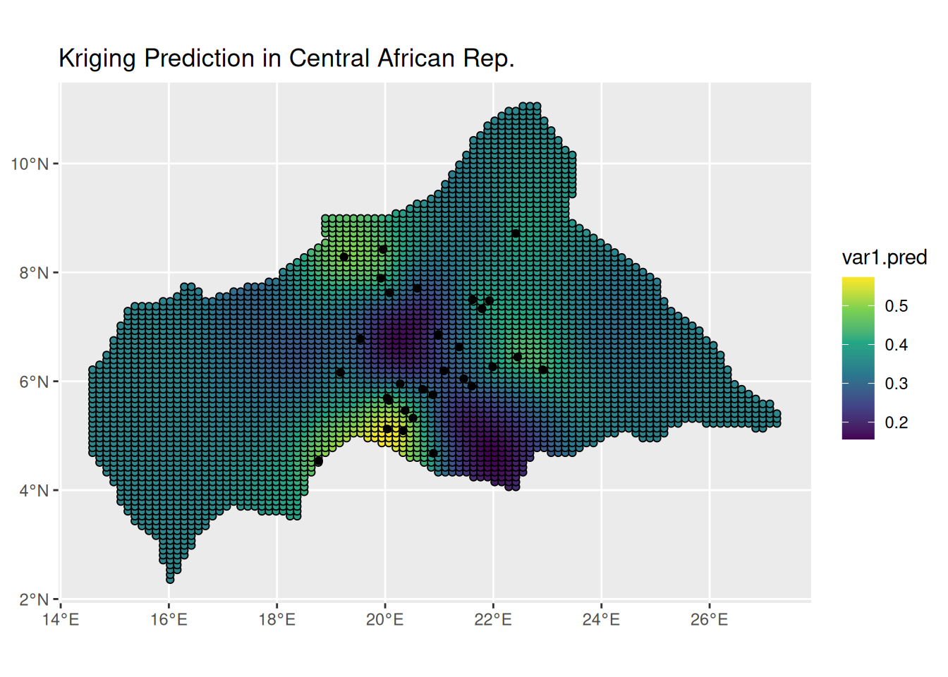
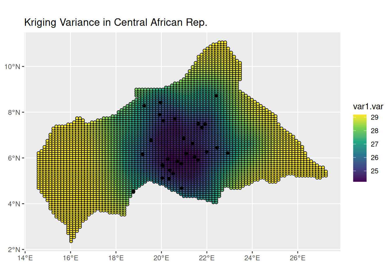
ggplot() +
  geom_sf(data = kpred,
          aes(fill = var1.var),
          shape=21, stroke=0.5) +
  geom_sf(data = infected_sf) +
  scale_fill_viridis_c() +
  labs(title = "Kriging Variance in Central African Rep.") +
  theme(legend.position = "right")