6.3.2 Example: Epidemic X

6.3.2.1 The SEIR Model

What happens if an infectious disease has an incubation period?

Scenario: simulate an epidemic to build an SEIR model (susceptible, exposed, infected, recovered).

How to use this in practice?

The {deSolve} package uses differential equations.

1. Define a function for the SEIR model and its parameters, where:

• $\beta$ is the transmission rate
• $\sigma$ is the rate of latent individuals becoming infectious
• $\gamma$ is the rate of recovery

SEIR <- function(time, state, parameters) {
  # variables need to be in a list
  with(as.list(c(state, parameters)), {
    # Parameters
    beta <- parameters[1] # Transmission rate
    sigma <- parameters[2] # Rate of latent individuals becoming infectious
    gamma <- parameters[3] # Rate of recovery

    # SEIR equations
    dS <- -beta * S * I / N
    dE <- beta * S * I / N - sigma * E
    dI <- sigma * E - gamma * I
    dR <- gamma * I

    # Return derivatives
    return(list(c(dS, dE, dI, dR)))
  })
}

2. Simulate starting parameters by assigning values.

N <- 1000 # Total population size
beta <- 0.3 # Transmission rate
sigma <- 0.1 # Rate of latent individuals becoming infectious
gamma <- 0.05 # Rate of recovery

3. Set an initial state and a time vector.

initial_state <- c(S = N - 1, E = 1, I = 0, R = 0)

# Time vector
times <- seq(0, 100, by = 1)

4. Use the ode() function from the deSolve package for solving the differential equations in the the SEIR model function created.

output <- deSolve::ode(y = initial_state,
                       times = times,
                       func = SEIR,
                       parms = c(beta = beta,
                                 sigma = sigma,
                                 gamma = gamma))

The output is a matrix. To convert to a data frame:

simulated_data <- as.data.frame(output)

head(simulated_data)

##   time        S         E          I           R
## 1    0 999.0000 1.0000000 0.00000000 0.000000000
## 2    1 998.9857 0.9186614 0.09324728 0.002384628
## 3    2 998.9452 0.8699953 0.17567358 0.009145043
## 4    3 998.8812 0.8483181 0.25070051 0.019828923
## 5    4 998.7954 0.8493639 0.32110087 0.034138118
## 6    5 998.6890 0.8699856 0.38915443 0.051899977

Plotting the simulated data of the SEIR model, with the number of susceptible, exposed, infectious, and recovered individuals over time.

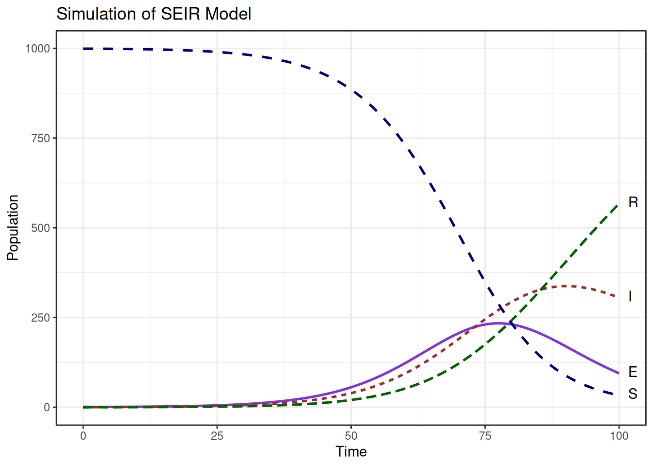
Plot shows how individuals interact with each other over time.