6.3.3 Example: Epidemic Y

6.3.3.1 INLA: an empirical Bayes approach to GAMs

Scenario: epidemic over 100 days based on temperature level and number of cases simulated with a random poisson distribution.

Model: INLA - integrated nested Laplace approximation model.

A deterministic algorithm for Bayesian inference.
Useful for fitting complex models (GAMs).
Alternative to Markov Chain Monte Carlo (MCMC).

Additional reading that may be useful: the R-INLA website, with tutorials and examples and a gentle INLA tutorial.

Install the INLA package (might take a while…)

Create the sample data.

set.seed(123)
epidemic_data <- data.frame(
  day = 1:100,
  temperature = rnorm(100, mean = 20, sd = 5),
  cases = rpois(100,
                lambda = 10 + sin(1:100 / 20) * 10 + rnorm(100, 
                                                           sd = 5)))

# View the first few rows of data
head(epidemic_data)

##   day temperature cases
## 1   1    17.19762    13
## 2   2    18.84911     8
## 3   3    27.79354     9
## 4   4    20.35254    11
## 5   5    20.64644     6
## 6   6    28.57532    14

Model the number of cases as a function of time and temperature
- non-linear effect of time using a random walk model (model = “rw2”)
- linear effect of temperature

# Define the model formula
formula <- cases ~ f(day, model = "rw2") + temperature

# Fit the model using INLA
result <- inla(formula,
               family = "poisson",
               data = epidemic_data)

Check the results:

result$summary.fixed

##                     mean          sd  0.025quant     0.5quant  0.975quant
## (Intercept)  2.389329032 0.144602391  2.10579390  2.389320218 2.672915611
## temperature -0.004819585 0.006762735 -0.01808339 -0.004818755 0.008439435
##                     mode          kld
## (Intercept)  2.389320552 3.237757e-11
## temperature -0.004818768 4.003960e-11

kld refers to Kullback and Leibler (1951).

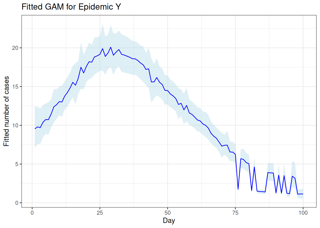
The predicted number of cases per day can be extracted and plotted:

time_effect <- result$summary.random$day

fitted_values <- result$summary.fitted.values

# Creating a data frame for plotting
plot_data <- data.frame(Day = epidemic_data$day,
                        FittedCases = fitted_values$mean,
                        Lower = fitted_values$`0.025quant`,
                        Upper = fitted_values$`0.975quant`)